Before we can treat “starters”, we have to introduce “FYE proxies”—estimates of the degree-granting engineering programs First-Year Engineering (FYE) students would have declared had they not been required to enroll in FYE.
Users of midfielddata practice data are not required to reproduce
this vignette—the results are included with midfieldr in the
fye_proxy data set.
This article in the MIDFIELD workflow:
- Planning
- Initial processing
- Blocs
- Ever-enrolled
- FYE proxies
- Starters
- Graduates
- Ever-enrolled
- Groupings
- Metrics
- Displays
Potential for starter miscounts
At some US institutions, engineering students are required to complete a First-Year Engineering (FYE) program as a prerequisite for declaring an engineering major. Administratively, degree-granting engineering programs such as Electrical Engineering or Mechanical Engineering treat their incoming post-FYE students as their “starting” cohorts. However, when computing a metric such as graduation rate that requires a count of starters, FYE records must be treated with special care to avoid a miscount.
To illustrate the potential for miscounting starters, suppose we wish to calculate a Mechanical Engineering (ME) graduation rate. Students starting in ME constitute the starting pool and the fraction of that pool graduating in ME is the graduation rate.
At FYE institutions, an ME program would typically define their starting pool as the post-FYE cohort entering their program. This may be the best information available, but it invariably undercounts starters by failing to account for FYE students who leave the institution or switch to non-engineering majors. In the absence of the FYE requirement some of these students would have been ME starters. By neglecting these students, the count of ME starters is artificially low resulting in an ME graduation rate that is artificially high. The same is true for every degree-granting engineering major in an FYE institution.
Because of the special nature of FYE programs, we cannot address starter miscounts by grouping FYE students with those admitted with “undecided” or “unknown” CIP codes—FYE students are neither. They were admitted as Engineering majors (2-digit CIP 14). We simply don’t know to which degree-granting program (6-digit CIP) they intended to transition.
Therefore, to avoid miscounting starters at FYE institutions, we estimate the 6-digit CIP codes of the degree-granting engineering programs that FYE students would have declared had they not been required to enroll in FYE.
Definitions
- FYE
-
First-Year Engineering program, a common-first-year curriculum that is a prerequisite for declaring an engineering major at some US institutions. Denoted by its own CIP code, FYE is not a degree-granting program.
- FYE proxy
-
Our estimate of the degree-granting engineering program in which an FYE student would have enrolled had they not been required to enroll in FYE. The proxy, a 6-digit CIP code, denotes the program of which the FYE student can be considered a starter.
- bloc
-
A grouping of student-level data dealt with as a unit, for example, starters, students ever-enrolled, graduates, transfer students, traditional and non-traditional students, migrators, etc.
- starters
-
Bloc of degree-seeking students in their initial terms enrolled in degree-granting programs.
- migrators
-
Bloc of students who leave one program to enroll in another. Also called switchers.
- multiple imputation
-
Method of imputing missing categorical data, in this case, imputing the FYE proxy 6-digit CIP codes.
Method
We apply prep_fye_mice() to the student and
term source files to construct a data frame suitable for
imputation using the mice R package. The procedure has four steps:
Use
prep_fye_mice()from the midfieldr package to estimate some of the FYE proxy CIPs, treat the remainder as missing values, and structure the data frame for imputation.Optional. If the default predictor variables (institution, race/ethnicity, and sex) do not meet the needs of your study, you can define your own.
Use
mice()from the mice package to impute the 6-digit CIP missing values.Post-processing to convert the results to useful form and to remove migrators.
Three outcomes are possible, depending on your goals and available data:
Use midfielddata practice data to recreate the
fye_proxydata set included with midfieldr—as we do in this vignette.Use midfielddata practice data to create an alternate set of FYE proxies based on a different random number seed or different predictor variables. The result would have the same IDs as
fye_proxybut different ID-proxy pairings.Use MIDFIELD research data and construct your own FYE proxies.
For a given set of source files, FYE proxies need be created only once and written to file. The result can be used as needed unless the source files change.
Reminder. midfielddata is for practice, not research.
Load data
Start. If you are writing your own script to follow along, we use these packages in this article:
library("midfieldr")
library("midfielddata")
library("data.table")
library("ggplot2")
library("mice")
Load. Practice datasets. View data dictionaries via
?student, ?term.
# Load practice data
data(student, term)
Loads with midfieldr. Prepared data, derived in Programs. View data
dictionary via ?study_programs.
study_programs
Initial processing
Unlike the initial processing in previous articles, we do not filter for data sufficiency and degree seeking.
Select (optional). Reduce the number of columns. Code reproduced from Getting started.
# Optional. Copy of source files with all variables
source_student <- copy(student)
source_term <- copy(term)

# Optional. Select variables required by midfieldr functions
student <- select_basic_cols(source_student)
term <- select_basic_cols(source_term)
prep_fye_mice()
The purpose of prep_fye_mice() is preparing a data frame
for the mice R package. Operates on the complete, unfiltered
student and term source data to create a data
frame with three predictor variables and an FYE proxy variable. The
values in proxy are determined by a student’s first
post-FYE program code, as follows:
Post-FYE in Engineering. The student completes FYE and enrolls in an engineering major. For this outcome, we know that at the student’s first opportunity, they enrolled in an engineering major of their choosing. The CIP code of that program is returned as the student’s FYE proxy.
Post-FYE not in Engineering. The student migrates to a non-engineering major or has no post-FYE records in the database. The data provide no indication of the student’s preferred degree-granting engineering major. Thus their FYE proxy value is returned as NA, to be treated as missing data to be imputed.
Arguments.
midfield_studentData frame of student observations, keyed by student ID. Default isstudent. Required variables aremcid,race, andsex. Use all rows of your sourcestudentdata table.midfield_termData frame of term observations keyed by student ID. Default isterm. Required variables aremcid,institution,term, andcip6. Use all rows of your sourcetermdata table.fye_codesOptional character vector of 6-digit CIP codes assigned to FYE programs. Default is “140102”. Argument to be used by name.
Implicit arguments. The following implementations yield identical results.
# Required arguments in order and explicitly named
x <- prep_fye_mice(midfield_student = student, midfield_term = term)

# Required arguments in order, but not named
y <- prep_fye_mice(student, term)

# Using the implicit defaults
z <- prep_fye_mice()

# Demonstrate equivalence
check_equiv_frames(x, y)
#> [1] TRUE
check_equiv_frames(x, z)
#> [1] TRUE
Output. The function returns one row per FYE student keyed
by student ID. All variables except ID are returned as factors to meet
the requirements of mice().
# Working data frame
DT <- prep_fye_mice(student, term)
DT
#>                 mcid   race    sex   institution  proxy
#>               <char> <fctr> <fctr>        <fctr> <fctr>
#>    1: MCID3111190643  Asian Female Institution J   <NA>
#>    2: MCID3111190747  Asian Female Institution J   <NA>
#>    3: MCID3111288144  Asian Female Institution J   <NA>
#>   ---
#> 5787: MCID3112328635  White   Male Institution J 143501
#> 5788: MCID3112328655  White   Male Institution J 143501
#> 5789: MCID3112382784  White   Male Institution J 143501
Missing data
The output of prep_fye_mive() should contain missing
values in the proxy column only. Other variables are complete. A
race/ethnicity or sex value of “unknown” is treated as an observed
value, not missing data. And while no values of ID or institution are
unknown or missing in this example, such observations (if they existed)
would have to be removed.
Checking that all variables except proxy are
complete.
# Number of unique IDs
x <- length(unique(DT$mcid))

# Number of complete cases on four variables
y <- sum(complete.cases(DT[, .(mcid, race, sex, institution)]))

# Demonstrate equivalence
all.equal(x, y)
#> [1] TRUE
Number of missing observations in proxy.
# Number NAs in proxy
sum(is.na(DT$proxy))
#> [1] 2152

# Percentage NAs in proxy
100 * round(sum(is.na(DT$proxy)) / nrow(DT), 3)
#> [1] 37.2
Missing at random (MAR). These missing proxy
data are caused by a student’s decision to migrate to a non-engineering
major or to leave the database. At the time of making that decision, the
FYE student would not yet have enrolled in a degree-granting engineering
major, thus their decision is unlikely to be related to any specific
engineering major.
That a CIP is missing, therefore, is unlikely to be related to a specific CIP value—but may be related to other observations such as institution, race/ethnicity, or sex. Missing data of this type are classified as “missing at random” (MAR) which are suitable for multiple imputation and yield unbiased results (Grace-Martin 2012).
Multiple imputation. Lastly, while 5–10 imputations are generally considered adequate for unbiasedness, Bodner (2008) recommends having as many imputations as the percentage of missing data.
# Number of proxies to be imputed
(N_impute <- sum(is.na(DT$proxy)))
#> [1] 2152

# Number of observations with complete predictor information
(N_complete <- sum(complete.cases(DT[, .(mcid, race, sex, institution)])))
#> [1] 5789

# Percent missing proxies
(percent_missing <- round(100 * N_impute / N_complete, 3))
#> [1] 37.174
As shown here, the overall percentage of missing data is 37.17%, suggesting we set the number of imputations to 37.
# For the "m" argument in mice()
(m_imputations <- round(percent_missing, 0))
#> [1] 37
Chart. The chart displays the percent missing data by
category. The institution category isn’t used because the
practice data contain FYE students in one institution only. The vertical
dashed line indicates the 37% percent missing data overall.
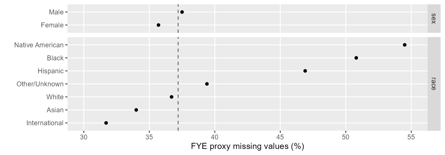
Figure 1: Percent missing data by category.
Setting up mice()
The mice package (van Buuren and Groothuis-Oudshoorn 2011) implements multiple imputation by chained equations (MICE). MICE is also known as “fully conditional specification” or “sequential regression multiple imputation” and is suitable for categorical variables such as ours (Azur et al. 2011). Our computational procedure follows the approach suggested by Dhana (2017).
Standard predictors
Framework. Our first use of mice() is to
examine the imputation framework by calling the function with zero
iterations on the DT data frame. mice()
produces a “multiply-imputed data set”, an R object of class “mids”.
# Imputation framework
framework <- mice(DT, maxit = 0)
#> Warning: Number of logged events: 2
framework
#> Class: mids
#> Number of multiple imputations:  5
#> Imputation methods:
#>        mcid        race         sex institution       proxy
#>          ""          ""          ""          ""   "polyreg"
#> PredictorMatrix:
#>             mcid race sex institution proxy
#> mcid           0    1   1           0     1
#> race           0    0   1           0     1
#> sex            0    1   0           0     1
#> institution    0    1   1           0     1
#> proxy          0    1   1           0     0
#> Number of logged events:  2
#>   it im dep     meth         out
#> 1  0  0     constant        mcid
#> 2  0  0     constant institution
Logged events warning. The printout above includes a warning about two “logged events”—an indication that two variables will not be used as predictors. We can isolate the warning for a closer look,
# Examine the warning
framework$loggedEvents
#>   it im dep     meth         out
#> 1  0  0     constant        mcid
#> 2  0  0     constant institution
The two variables are mcid and
institution.
mcidwas never intended to be a predictor variable. We retain the ID column so that imputed CIP values are assigned to specific IDs.institutionusually is a predictor. In this case, however, the FYE students are all at the same institution—a characteristic of the midfielddata practice data only.
Imputation methods. We look more closely at two elements of this framework. The first is the imputation method vector.
# Imputation method
method_vector <- framework[["method"]]
method_vector
#>        mcid        race         sex institution       proxy
#>          ""          ""          ""          ""   "polyreg"
The “polyreg” imputation method (polytomous logistic regression) is
appropriate for data, like ours, comprising unordered categorical
variables. Variable proxy is imputed using the polyreg
method; the other variables, being predictors, are not imputed, thus
their methods are empty.
Had the method not been correctly assigned, we would assign it as follows,
# Manually assign the variable(s) being imputed
method_vector[c("proxy")] <- "polyreg"

# Manually assign the variable(s) not being imputed
method_vector[c("mcid", "institution", "race", "sex")] <- ""
method_vector
#>        mcid        race         sex institution       proxy
#>          ""          ""          ""          ""   "polyreg"
Predictor matrix. The second element to review is the predictor matrix. A row label identifies the variable being predicted; the columns indicate the predictor variables.
# Imputation predictor matrix
predictor_matrix <- framework[["predictorMatrix"]]
predictor_matrix
#>             mcid race sex institution proxy
#> mcid           0    1   1           0     1
#> race           0    0   1           0     1
#> sex            0    1   0           0     1
#> institution    0    1   1           0     1
#> proxy          0    1   1           0     0
However, only those variables assigned a method are imputed. In our
case, the only variable to be imputed is proxy, so the only
row of this matrix that gets used is the last row.
# Predictor row for this example
predictor_matrix["proxy", ]
#>        mcid        race         sex institution       proxy
#>           0           1           1           0           0
The zeros and ones tell us that proxy is going to be
predicted by race and sex. Again, the institution variable is not a
predictor because the practice data contain one FYE institution only.
(This would not be the case if one were using the MIDFIELD research
database.)
Had the default setting been incorrect, we can set them manually.
Again, note that the bottom row is the only row we need because only the
proxy variable is being imputed.
# Manually assign zero columns
predictor_matrix[, c("mcid", "proxy", "institution")] <- 0

# Manually assign predictor columns
predictor_matrix[, c("race", "sex")] <- c(0, 0, 0, 0, 1)
predictor_matrix
#>             mcid race sex institution proxy
#> mcid           0    0   0           0     0
#> race           0    0   0           0     0
#> sex            0    0   0           0     0
#> institution    0    0   0           0     0
#> proxy          0    1   1           0     0
If the data included more than one FYE institution, the manual assignment would be,
Optional predictors
The default predictors set up by prep_fye_mice() are
institution (required), race/ethnicity, and sex. If these are
acceptable, you can skip to the next section, Imputing missing values.
Predictors can be edited or added before invoking
mice(). As before, ensure that the only missing values are
in the proxy column. Other variables are expected to be complete (no NA
values). A value of “unknown” in a predictor column, e.g.,
race/ethnicity or sex, is an acceptable value, not missing data.
Observations with missing or unknown values in the ID or institution
columns should be removed.
For example, suppose we wish to replace race/ethnicity and sex with a
people variable that has four possible values
(Domestic Female, Domestic Male,
International Female, and International Male)
where “domestic” means a US citizen; and we want to add a variable that
encodes the year of a student’s first term in FYE.
Creating variables. Remove any unknown observations of
race/ethnicity and sex to create the desired people
variable.
# Data frame to illustrate optional predictors
opt_DT <- copy(DT)

# Factor to character
cols_to_edit <- c("race", "sex")
opt_DT[, (cols_to_edit) := lapply(.SD, as.character), .SDcols = cols_to_edit]

# Filter unknown race and sex
opt_DT <- opt_DT[sex != "Unknown"]
opt_DT <- opt_DT[race != "Other/Unknown"]

# Create origin variable
opt_DT[, origin := fcase(
  race != "International", "Domestic",
  race == "International", "International",
  default = NA_character_
)]
opt_DT <- opt_DT[!is.na(origin)]

# Create people variable
opt_DT[, people := paste(origin, sex)]
opt_DT[, people := as.factor(people)]
opt_DT[, c("race", "sex", "origin") := NULL]

# Display result
setcolorder(opt_DT, c("mcid", "people", "institution", "proxy"))
opt_DT
#>                 mcid          people   institution  proxy
#>               <char>          <fctr>        <fctr> <fctr>
#>    1: MCID3111190643 Domestic Female Institution J   <NA>
#>    2: MCID3111190747 Domestic Female Institution J   <NA>
#>    3: MCID3111288144 Domestic Female Institution J   <NA>
#>   ---
#> 5569: MCID3112328635   Domestic Male Institution J 143501
#> 5570: MCID3112328655   Domestic Male Institution J 143501
#> 5571: MCID3112382784   Domestic Male Institution J 143501
Check the unique values.
# Display unique people
sort(unique(opt_DT$people))
#> [1] Domestic Female      Domestic Male        International Female
#> [4] International Male
#> 4 Levels: Domestic Female Domestic Male ... International Male
Adding a variable. Obtain the student’s first term in the
data set from the term data table using a left-outer
join.
# Add all term variables by ID
cols_to_join <- term[, .(mcid, term)]
opt_DT <- cols_to_join[opt_DT, on = c("mcid")]

# Filter for first term
setkeyv(opt_DT, c("mcid", "term"))
opt_DT <- opt_DT[, .SD[1], by = c("mcid")]

# Create year variable
opt_DT[, year := substr(term, 1, 4)]
opt_DT[, year := as.factor(year)]
opt_DT[, term := NULL]

# Display result
setcolorder(opt_DT, c("mcid", "people", "institution", "year", "proxy"))
opt_DT
#> Key: <mcid>
#>                 mcid             people   institution   year  proxy
#>               <char>             <fctr>        <fctr> <fctr> <fctr>
#>    1: MCID3111142290      Domestic Male Institution J   1988 141001
#>    2: MCID3111142294      Domestic Male Institution J   1988 141001
#>    3: MCID3111142961 International Male Institution J   1988 142101
#>   ---
#> 5569: MCID3112447659      Domestic Male Institution J   2009   <NA>
#> 5570: MCID3112447663      Domestic Male Institution J   2009   <NA>
#> 5571: MCID3112447664      Domestic Male Institution J   2009   <NA>
Filtering. Ensure complete cases except in
proxy.
# Identify complete cases in predictor variables
rows_we_want <- complete.cases(opt_DT[, .(mcid, people, institution, year)])

# Filter for complete predictors
opt_DT <- opt_DT[rows_we_want]
opt_DT
#> Key: <mcid>
#>                 mcid             people   institution   year  proxy
#>               <char>             <fctr>        <fctr> <fctr> <fctr>
#>    1: MCID3111142290      Domestic Male Institution J   1988 141001
#>    2: MCID3111142294      Domestic Male Institution J   1988 141001
#>    3: MCID3111142961 International Male Institution J   1988 142101
#>   ---
#> 5569: MCID3112447659      Domestic Male Institution J   2009   <NA>
#> 5570: MCID3112447663      Domestic Male Institution J   2009   <NA>
#> 5571: MCID3112447664      Domestic Male Institution J   2009   <NA>
Framework for optional predictors.
# Imputation framework
opt_framework <- mice(opt_DT, maxit = 0)
#> Warning: Number of logged events: 2
opt_framework
#> Class: mids
#> Number of multiple imputations:  5
#> Imputation methods:
#>        mcid      people institution        year       proxy
#>          ""          ""          ""          ""   "polyreg"
#> PredictorMatrix:
#>             mcid people institution year proxy
#> mcid           0      1           0    1     1
#> people         0      0           0    1     1
#> institution    0      1           0    1     1
#> year           0      1           0    0     1
#> proxy          0      1           0    1     0
#> Number of logged events:  2
#>   it im dep     meth         out
#> 1  0  0     constant        mcid
#> 2  0  0     constant institution
Imputation method for optional predictors.
# Imputation framework
opt_method_vector <- opt_framework[["method"]]
opt_method_vector
#>        mcid      people institution        year       proxy
#>          ""          ""          ""          ""   "polyreg"
Predictor matrix for optional predictors.
# Imputation predictor matrix
opt_predictor_matrix <- opt_framework[["predictorMatrix"]]
opt_predictor_matrix
#>             mcid people institution year proxy
#> mcid           0      1           0    1     1
#> people         0      0           0    1     1
#> institution    0      1           0    1     1
#> year           0      1           0    0     1
#> proxy          0      1           0    1     0
Percent missing data for setting the number of multiple imputations.
Imputing missing values
The three essential arguments for mice() are the
DT data frame, the method_vector, and the
predictor_matrix. The number of multiple imputations
m is set to 37 as discussed in Missing data. Setting
printFlag = TRUE displays progress in the console.
The default seed argument is NULL, but by setting the
seed as shown the vignette results are reproducible.
For the practice data, 5 iterations of 37 imputations takes about 3 minutes (depending on your machine). For MIDFIELD research data, however, imputation runs significantly longer.
# Impute missing proxy data
DT_mids <- mice(
  data = DT,
  m = m_imputations,
  maxit = 5, # default
  method = method_vector,
  predictorMatrix = predictor_matrix,
  seed = 20180624,
  printFlag = TRUE
)
# output in console with printFlag = TRUE
# >  iter imp variable
# >   1   1  proxy
# >   1   2  proxy
# >   1   3  proxy
# >   1   4  proxy
# >   1   5  proxy
# >   ---
# >   5  33  proxy
# >   5  34  proxy
# >   5  35  proxy
# >   5  36  proxy
# >   5  37  proxy
Post-processing
Extracting the result. We apply
mice::complete() to extract the data from the
mids object. The missing data have been replaced by imputed
values.
# Revert to default random number generation
set.seed(NULL)

# Extract data from the mids object
DT <- mice::complete(DT_mids)

# Convert to data.table structure
setDT(DT)
DT <- DT[order(mcid)]
DT
#>                 mcid          race    sex   institution  proxy
#>               <char>        <fctr> <fctr>        <fctr> <fctr>
#>    1: MCID3111142290         Asian   Male Institution J 141001
#>    2: MCID3111142294         Asian   Male Institution J 141001
#>    3: MCID3111142961 International   Male Institution J 142101
#>   ---
#> 5787: MCID3112447659         White   Male Institution J 141901
#> 5788: MCID3112447663         White   Male Institution J 140201
#> 5789: MCID3112447664         White   Male Institution J 141001
Selecting columns. To use the result, we need only two columns: IDs and the the predicted starting programs.
# Subset the data
DT <- DT[, .(mcid, proxy)]
DT
#>                 mcid  proxy
#>               <char> <fctr>
#>    1: MCID3111142290 141001
#>    2: MCID3111142294 141001
#>    3: MCID3111142961 142101
#>   ---
#> 5787: MCID3112447659 141901
#> 5788: MCID3112447663 140201
#> 5789: MCID3112447664 141001
Recoding. We convert the CIP codes from factor to character.
# Convert factors
DT[, proxy := as.character(proxy)]
DT
#>                 mcid  proxy
#>               <char> <char>
#>    1: MCID3111142290 141001
#>    2: MCID3111142294 141001
#>    3: MCID3111142961 142101
#>   ---
#> 5787: MCID3112447659 141901
#> 5788: MCID3112447663 140201
#> 5789: MCID3112447664 141001
Filtering. Proxies are substitutes for students starting in FYE. Thus we filter to remove migrators, retaining the proxies of first-term FYE students only.
# Order term data by ID and term
ordered_term <- term[, .(mcid, term, cip6)]
setorderv(ordered_term, cols = c("mcid", "term"))

# Obtain first term of all students
first_term <- ordered_term[, .SD[1], by = c("mcid")]

# Reduce to first term in FYE
first_term_fye_mcid <- first_term[cip6 == "140102", .(mcid)]

# Inner join to remove migrators from working data frame
DT <- first_term_fye_mcid[DT, on = c("mcid"), nomatch = NULL]
setkey(DT, NULL)
DT
#>                 mcid  proxy
#>               <char> <char>
#>    1: MCID3111142290 141001
#>    2: MCID3111142294 141001
#>    3: MCID3111142961 142101
#>   ---
#> 4621: MCID3112447659 141901
#> 4622: MCID3112447663 140201
#> 4623: MCID3112447664 141001
Verify prepared data. To avoid deriving this data frame
each time it is needed in other vignettes, the same information is
provided in the fye_proxy data frame included with
midfieldr. Here we verify that the two data frames have the same
content.
# Demonstrate equivalence
check_equiv_frames(DT, fye_proxy)
#> [1] TRUE
Assessing FYE proxies
Credibility
Here we summarize the FYE proxy data set to see how many students our algorithm assigned to which engineering majors. Start by extracting the unique set of CIP codes from the proxy data set.
# Identify unique CIP codes in the proxy data
proxy_cips <- sort(unique(fye_proxy$proxy))
proxy_cips
#>  [1] "140201" "140301" "140701" "140801" "140901" "141001" "141101" "141401"
#>  [9] "141801" "141901" "142101" "143301" "143501"
Obtain the program names from the cip data set (provided
with midfieldr). We use the 4-digit names that in engineering generally
represent department-level programs.
# Obtain the 4-digit program names corresponding to these codes
proxy_program_names <- filter_programs(cip, proxy_cips)
proxy_program_names <- proxy_program_names[, .(cip6, program = cip4name)]
proxy_program_names
#>       cip6                                                 program
#>     <char>                                                  <char>
#>  1: 140201   Aerospace, Aeronautical and Astronautical Engineering
#>  2: 140301 Agricultural, Biological Engineering and Bioengineering
#>  3: 140701                                    Chemical Engineering
#>  4: 140801                                       Civil Engineering
#>  5: 140901                           Computer Engineering, General
#>  6: 141001  Electrical, Electronics and Communications Engineering
#>  7: 141101                                   Engineering Mechanics
#>  8: 141401         Environmental, Environmental Health Engineering
#>  9: 141801                                   Materials Engineering
#> 10: 141901                                  Mechanical Engineering
#> 11: 142101                          Mining and Mineral Engineering
#> 12: 143301                                Construction Engineering
#> 13: 143501                                  Industrial Engineering
Join these names to the proxy data set, summarize by program, and order the rows by descending N.
# Join these program names to the proxy data
proxy_programs <- proxy_program_names[fye_proxy[, .(cip6 = proxy)], .(program), on = c("cip6")]

# Count by program and order rows in descending magnitude
proxy_programs <- proxy_programs[, .N, by = c("program")]
setorderv(proxy_programs, order = -1, cols = c("N"))
proxy_programs
#>                                                     program     N
#>                                                      <char> <int>
#>  1:                                  Mechanical Engineering  1048
#>  2:  Electrical, Electronics and Communications Engineering   673
#>  3:                                       Civil Engineering   592
#>  4:                           Computer Engineering, General   565
#>  5:   Aerospace, Aeronautical and Astronautical Engineering   511
#>  6:                                  Industrial Engineering   395
#>  7:                                    Chemical Engineering   365
#>  8:                                   Engineering Mechanics   136
#>  9:                          Mining and Mineral Engineering   134
#> 10:                                   Materials Engineering   103
#> 11: Agricultural, Biological Engineering and Bioengineering    82
#> 12:                                Construction Engineering    18
#> 13:         Environmental, Environmental Health Engineering     1
For comparison, the National Science Foundation (NSF) reports that in 2012, the top seven US engineering majors ranked by enrollment were (SEI dashboard 2014):
- Mechanical
- Electrical
- Civil
- Chemical
- Industrial
- Aerospace
- Materials
In Table 1, we show the FYE proxy programs and indicate the equivalent NSF ranking cited above. The assignment of proxies is fairly consistent with the NSF results, though the practice data have a higher frequency of aerospace proxies than expected. Recall that the practice data contain only three institutions while the NSF information is based on nearly 3000 US undergraduate institutions (SEI report 2014).
| Program | NSF ranking | N |
|---|---|---|
| Mechanical Engineering | 1 | 1048 |
| Electrical, Electronics and Communications Engineering | 2 | 673 |
| Civil Engineering | 3 | 592 |
| Computer Engineering, General | 565 | |
| Aerospace, Aeronautical and Astronautical Engineering | 6 | 511 |
| Industrial Engineering | 5 | 395 |
| Chemical Engineering | 4 | 365 |
| Engineering Mechanics | 136 | |
| Mining and Mineral Engineering | 134 | |
| Materials Engineering | 7 | 103 |
| Agricultural, Biological Engineering and Bioengineering | 82 | |
| Construction Engineering | 18 | |
| Environmental, Environmental Health Engineering | 1 |
We conclude that the imputation is credible at least to the extent that the ranking of the majors is generally consistent with expectations.
Quantifying potential miscounts
The main goal of estimating FYE proxies is to prevent starter miscounts. Here, we assess the potential for miscounts if FYE records are not treated as recommended.
We start with the first_term data frame created earlier
(in Post-processing) containing the
initial term information of all students in the practice data.
# First term of all students
first_term
#> Index: <cip6>
#>                  mcid   term   cip6
#>                <char> <char> <char>
#>     1: MCID3111142225  19881 140901
#>     2: MCID3111142283  19881 240102
#>     3: MCID3111142290  19881 140102
#>    ---
#> 97553: MCID3112898894  20181 451001
#> 97554: MCID3112898895  20181 302001
#> 97555: MCID3112898940  20181 050103
Identify starters, including FYE proxies, in the four case study programs. (This procedure is more fully developed in the Starters vignette.)
# Join proxies by ID (left join) to first-term data
start <- fye_proxy[first_term, .(mcid, cip6, proxy), on = c("mcid")]

# Distinguish FYE from direct matriculants
start[, matric := fcase(
  is.na(proxy), "direct",
  !is.na(proxy), "fye"
)]

# Create start variable
start[, start := fcase(
  matric == "fye", proxy,
  matric == "direct", cip6
)]

# Filter to retain case study program starters
join_labels <- copy(study_programs)
setnames(join_labels, old = "cip6", new = "start")
start <- join_labels[start, on = c("start")]
start <- start[!is.na(program)]

# Display result
start[order(matric, start)]
#>        start program           mcid   cip6  proxy matric
#>       <char>  <char>         <char> <char> <char> <char>
#>    1: 140801      CE MCID3111170903 140801   <NA> direct
#>    2: 140801      CE MCID3111170949 140801   <NA> direct
#>    3: 140801      CE MCID3111174233 140801   <NA> direct
#>   ---
#> 5382: 143501     ISE MCID3112447549 140102 143501    fye
#> 5383: 143501     ISE MCID3112447596 140102 143501    fye
#> 5384: 143501     ISE MCID3112447600 140102 143501    fye
This data frame contains all direct-matriculation starters in the case study programs plus the FYE students with one of these programs as their estimated proxy.
Grouping by program and type of matriculation, we can determine the FYE percentage of all starters.
# Summarize
start <- start[, .N, by = c("matric", "program")]

# Transform to row-record form
start <- dcast(start, program ~ matric, value.var = "N")

# Compute FYE as fraction of total
start[, N_starters := direct + fye]
start[, fye_pct := round(100 * fye / N_starters, 1)]
start
#> Key: <program>
#>    program direct   fye N_starters fye_pct
#>     <char>  <int> <int>      <int>   <num>
#> 1:      CE    714   592       1306    45.3
#> 2:      EE    669   673       1342    50.1
#> 3:     ISE     12   395        407    97.1
#> 4:      ME   1281  1048       2329    45.0
The results indicate (for the case study data) a potential under-count of 45% to 97% if FYE proxies are excluded when counting starters.