Graduation rate

Graduation rate is a widely used, though flawed, measure of academic achievement.

The American Council on Education estimates that the conventional definition of graduation rate may exclude up to 60% of students at 4-year institutions (Cook and Hartle 2011). Nevertheless, as Cook and Hartle explain,

… in the eyes of the public, policy makers, and the media, graduation rate is a clear, simple, and logical—if often misleading—number.

Recognizing that graduation rate is a popular metric, we propose a definition of graduation rate that includes all conventionally excluded students except migrators. You can skip the FYE content in this vignette if your study includes no FYE-style Engineering programs.

This vignette in the MIDFIELD workflow.

1. Planning
   
2. Initial processing
   
3. Blocs
   
4. Groupings
   
5. Metrics
   • Graduation rate
     
   • Stickiness
     
6. Displays

Definitions

graduation rate

Graduation rate \((G)\) is the ratio of the number of program “starter-graduates” \((N_{sg})\) (i.e., graduates from the program in which they started) to the number of program starters \((N_s)\). \[ G=\frac{N_{sg}}{N_s} \]

bloc

A grouping of student-level data dealt with as a unit, for example, starters, students ever-enrolled, graduates, transfer students, traditional and non-traditional students, migrators, etc.

starters

Bloc of degree-seeking students in their initial terms enrolled in degree-granting programs.

starter-graduates

Subset of the starters bloc who are graduates (timely completers) from their starting programs.

timely completion criterion

Completing a program in no more than a specified span of years, in many cases, within 6 years after admission (150% of the “normal” 4-year span), or possibly less for some transfer students.

migrators

Bloc of students who leave one program to enroll in another. Also called switchers.

undecided/unspecified

The MIDFIELD taxonomy includes the non-IPEDS code (CIP 999999) for Undecided or Unspecified indicating instances in which a student has not declared a major or an institution had not recorded a program.

Starters and migrators

As they pertain to the graduation rate metric, relationships among starters, migrators, and graduates (timely completers) of a given program P are illustrated in Figure 1.

• The overall rectangle represents the set of students ever enrolled in program P.

• The interior rectangle represents the set of graduates (timely completers) of program P.

• Region 1 (shaded) represents the graduation rate denominator \((N_s)\), the set of starters in program P.

• Region 2 (shaded) represents the graduation rate numerator \((N_{sg})\), the subset of starters who are also graduates of program P.

• Region 3 (unshaded) represents the set of students excluded from the graduation rate metric, depending on how “program” is defined as discussed below.

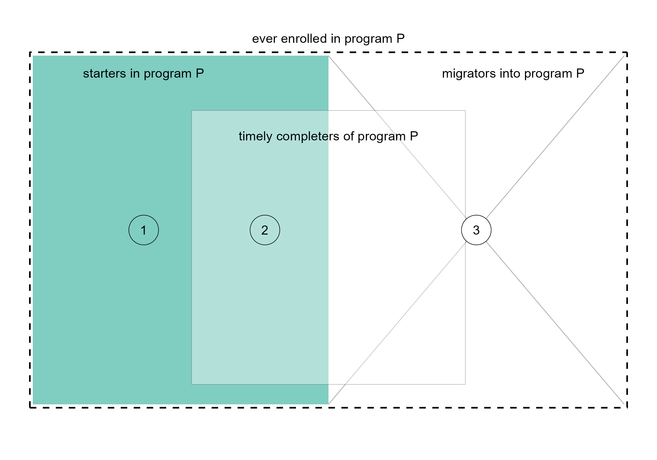
Figure 1. Graduation rate metric. Starters, migrators, and timely completers.

When calculating graduation rate, whether migrator-graduates are included in the count of graduates depends how a program is defined in terms of CIP codes.

• Institution level. Graduation rate computed at the institution level includes all migrators within the institution. For example, starters in Engineering (CIP 14) who graduate in Business (CIP 52) are both starters and timely completers at the institution level. IPEDS defines this rate as the institution completion rate.

• 2-digit CIP. Graduation rate includes migrator graduates within the same 2-digit CIP. For example, starters in Engineering (CIP 14) graduating in Business (CIP 52) are excluded from the count of Business graduates, but migrators within Engineering (all 6-digit CIP codes starting with 14) are both starters and timely completers in Engineering.

• 4-digit CIP. Similar to the 2-digit case. For example, starters in Electrical Engineering (CIP 1410) graduating in Mechanical Engineering (CIP 1419) are excluded from the count of Mechanical Engineering graduates, but migrators within Electrical Engineering (all 6-digit CIP codes starting with 1410) are both starters and timely completers in Electrical Engineering.

• 6-digit CIP. Rarely used. Graduation rate at this CIP level excludes all migrators from the count of graduates.

• Multiple CIPs. In some cases, a single program or major includes different 4-digit CIPs. For example, migrators between Systems Engineering (CIP 1427), Industrial Engineering (CIP 1435), Manufacturing Engineering (CIP 1436), and Operations Research (CIP 1437) might be considered both starters and timely completers in a general program of Industrial & Systems Engineering.

Who is a starter?

In the US, the predominant definition of graduation rate is that established by the US Department of Education, Integrated Postsecondary Education Data System (IPEDS). The IPEDS definition underlies the finding cited earlier that a graduation rate metric may exclude up to 60% of students.

Many of the IPEDS exclusions relate to how starters are defined. By expanding the starters definition, MIDFIELD proposes a graduation rate definition that includes all conventionally excluded students except migrators.

graduation rate (IPEDS)

The fraction of a cohort of full-time, first-time, degree-seeking undergraduates who complete their program within a percentage (100%, 150%, or 200%) of the “normal” time (typically 4 years) as defined by the institution. IPEDS excludes students who attend college part-time, who transfer between institutions, and who start in Winter or Spring terms (NCES-IPEDS 2020).

graduation rate (MIDFIELD)

The fraction of a cohort of degree-seeking undergraduates who complete their program in a timely manner (typically 6 years). MIDFIELD includes students who attend college part-time, who transfer between institutions, and who start in any term. Table 1 summarizes the comparison between the IPEDS and MIDFIELD graduation rate definitions.

Table 1: Comparing graduation rate definitions

Item	IPEDS	MIDFIELD	MIDFIELD notes
completion span:	4, 6, or 8 years	4, 6, or 8 years	Typical usage is 6 years
students admitted in:	Summer/Fall only	any term
part-time students are:	excluded	included	Timely completion same as full-time students
transfer students are:	excluded	included	Timely completion span adjusted for level at entry

First-Year Engineering (FYE) starters

We estimate the degree-granting engineering program in which an FYE student would have enrolled had they not been required to enroll in FYE. The FYE proxy, a 6-digit CIP code, denotes the program of which the FYE student can be considered a starter. For additional details, see the vignette FYE proxies.

Method

Demonstrating the following elements of a MIDFIELD workflow.

1. Planning.   The metric is graduation rate. Required blocs are starters and the subset of starters who graduate in their starting major. Grouping variables are program, race/ethnicity, and sex. Programs are the four Engineering programs used throughout.

2. Initial processing.   Filter the student-level records for data sufficiency and degree-seeking.

3. Blocs.   Gather starters, filter by program. Gather graduates, filter by program, filter by starters’ IDs and programs.

4. Groupings.   Add grouping variables.

5. Metrics   Summarize by grouping variables and compute graduation rate.

6. Displays   Create multiway chart and results table.

Reminder.   midfielddata datasets are for practice, not research.

Load data

Start.   If you are writing your own script to follow along, we use these packages in this article:

library(midfieldr)
library(midfielddata)
library(data.table)
library(ggplot2)

Load.   Practice datasets. View data dictionaries via ?student, ?term, ?degree.

# Load practice data
data(student, term, degree)

Loads with midfieldr.   Prepared data. View data dictionaries via ?study_programs, ?baseline_mcid, ?fye_proxy.

• study_programs (derived in Programs).

• baseline_mcid (derived in Blocs).

• fye_proxy (derived in FYE proxies).

Initial processing

Select (optional).   Reduce the number of columns. Code reproduced from Getting started.

# Optional. Copy of source files with all variables
source_student <- copy(student)
source_term <- copy(term)
source_degree <- copy(degree)

# Optional. Select variables required by midfieldr functions
student <- select_required(source_student)
term <- select_required(source_term)
degree <- select_required(source_degree)

Initialize.   From term and student, construct a data frame of student IDs filtered for data sufficiency and degree seeking as described in Blocs.

# Working data frame
DT <- copy(baseline_mcid)
DT
#>                  mcid
#>     1: MCID3111142689
#>     2: MCID3111142782
#>     3: MCID3111142881
#>    ---               
#> 76873: MCID3112785480
#> 76874: MCID3112800920
#> 76875: MCID3112870009

Starters

Starters.   The summary code chunk from Starters

# Isolate starting term
DT <- term[DT, .(mcid, term, cip6), on = c("mcid")]
DT <- DT[!cip6 %like% "999999"]
setorderv(DT, cols = c("mcid", "term"))
DT <- DT[, .SD[which.min(term)], by = "mcid"]
DT <- DT[, .(mcid, cip6)]
DT <- unique(DT)

# Continue for starters with FYE
DT <- fye_proxy[DT, .(mcid, cip6, proxy), on = c("mcid")]
DT[, start := fcase(
  cip6 == "140102", proxy,
  cip6 != "140102", cip6
)]
DT <- DT[, .(mcid, start)]

# Filter by program on start
join_labels <- copy(study_programs)
join_labels <- join_labels[, .(program, start = cip6)]
DT <- join_labels[DT, on = c("start"), nomatch = NULL]
DT[, start := NULL]
DT <- unique(DT)

Copy.   To prepare for joining with graduates.

# Prepare for joining
setcolorder(DT, c("mcid"))
starters <- copy(DT)
starters
#>                 mcid program
#>    1: MCID3111142965      EE
#>    2: MCID3111145102      EE
#>    3: MCID3111150194     ISE
#>   ---                       
#> 4051: MCID3112619118      EE
#> 4052: MCID3112619484      EE
#> 4053: MCID3112619666      ME

Graduates

Initialize.   The data frame of baseline IDs is the intake for this section.

# Working data frame
DT <- copy(baseline_mcid)

Graduates   The summary code chunk from Graduates

# Gather graduates, degree CIPs and terms
DT <- add_timely_term(DT, term)
DT <- add_completion_status(DT, degree)
DT <- DT[completion_status == "timely"]
DT <- degree[DT, .(mcid, term_degree, cip6), on = c("mcid")]

# Filter by programs and first degree terms
DT <- study_programs[DT, on = c("cip6"), nomatch = NULL]
DT <- DT[, .SD[which.min(term_degree)], by = "mcid"]
DT[, c("cip6", "term_degree") := NULL]
DT <- unique(DT)
DT
#>                 mcid program
#>    1: MCID3111142965      EE
#>    2: MCID3111145102      EE
#>    3: MCID3111146537      EE
#>   ---                       
#> 3262: MCID3112618976      ME
#> 3263: MCID3112619484      EE
#> 3264: MCID3112641535      ME

Starter-graduates

This section introduces new material—not adapted from the reusable code sections of other vignettes.

For a graduation rate metric, a timely completer is counted among the graduates only if they start and complete the same program.

Filter.   Use an inner join to filter the graduates by ID and program to match the IDs and programs of starters.

# Starter-graduates
DT <- starters[DT, on = c("mcid", "program"), nomatch = NULL]

Copy.   To prepare for joining with starters.

# Prepare for joining
setcolorder(DT, c("mcid"))
graduates <- copy(DT)
graduates
#>                 mcid program
#>    1: MCID3111142965      EE
#>    2: MCID3111145102      EE
#>    3: MCID3111150194     ISE
#>   ---                       
#> 1787: MCID3112617717      ME
#> 1788: MCID3112618976      ME
#> 1789: MCID3112619484      EE

Closer look

Examining the records of selected students in detail.

Example 1.   The student is a starter and a timely completer in Industrial/Systems Engineering (ISE). They appear in both blocs.

# Same ID in different blocs
mcid_we_want <- "MCID3111150194"
starters[mcid == mcid_we_want]
#>              mcid program
#> 1: MCID3111150194     ISE

graduates[mcid == mcid_we_want]
#>              mcid program
#> 1: MCID3111150194     ISE

Example 2.   The student is a starter in Electrical Engineering (EE). They are excluded from the graduation rate starter-graduate bloc because they did not complete EE. From degree we find that they completed CIP 143501 (ISE), one of the study programs. They are also excluded from a count of ISE graduates because they weren’t a ISE starter.

# Same ID in different blocs
mcid_we_want <- "MCID3111235261"
starters[mcid == mcid_we_want]
#>              mcid program
#> 1: MCID3111235261      EE

graduates[mcid == mcid_we_want]
#> Empty data.table (0 rows and 2 cols): mcid,program

degree[mcid == mcid_we_want, .(mcid, cip6)]
#>              mcid   cip6
#> 1: MCID3111235261 143501

Example 3.   The student is a starter in Civil Engineering (CE). They are excluded from the graduation rate starter-graduate bloc because they did not complete CE. From degree we find that they completed CIP 521401 (Marketing). They would also be excluded from a count of Marketing graduates because they weren’t a Marketing starter.

# Same ID in different blocs
mcid_we_want <- "MCID3111158691"
starters[mcid == mcid_we_want]
#>              mcid program
#> 1: MCID3111158691      CE

graduates[mcid == mcid_we_want]
#> Empty data.table (0 rows and 2 cols): mcid,program

degree[mcid == mcid_we_want, .(mcid, cip6)]
#>              mcid   cip6
#> 1: MCID3111158691 521401

Groupings

One of our grouping variables (program) is already included in the data frames. The next grouping variable is bloc to distinguish starters from graduates when the two data frames are combined.

Add a variable.   Label starters and graduates.

# For grouping by bloc
starters[, bloc := "starters"]
graduates[, bloc := "graduates"]

Join.   Combine the two blocs to prepare for summarizing. A student starting and graduating in the same program now has two observations in these data: one as a starter and one as a graduate.

# Prepare for summarizing
DT <- rbindlist(list(starters, graduates))
DT
#>                 mcid program      bloc
#>    1: MCID3111142965      EE  starters
#>    2: MCID3111145102      EE  starters
#>    3: MCID3111150194     ISE  starters
#>   ---                                 
#> 5840: MCID3112617717      ME graduates
#> 5841: MCID3112618976      ME graduates
#> 5842: MCID3112619484      EE graduates

Add variables.   Demographics from Groupings

# Join race/ethnicity and sex
cols_we_want <- student[, .(mcid, race, sex)]
DT <- cols_we_want[DT, on = c("mcid")]
DT
#>                 mcid          race  sex program      bloc
#>    1: MCID3111142965 International Male      EE  starters
#>    2: MCID3111145102         White Male      EE  starters
#>    3: MCID3111150194         Black Male     ISE  starters
#>   ---                                                    
#> 5840: MCID3112617717 International Male      ME graduates
#> 5841: MCID3112618976         White Male      ME graduates
#> 5842: MCID3112619484         White Male      EE graduates

Note.   MIDFIELD research findings are regularly grouped by program, race/ethnicity, and sex. However, applied to the practice data these groupings produce several groups with totals below the threshold we impose to preserve anonymity, introducing a number of NA values in the resulting charts and tables. These NAs are largely an artifact of applying these groupings to practice data.

Graduation rate

Summarize.   Count the numbers of observations for each combination of the grouping variables.

# Count observations by group
grouping_variables <- c("bloc", "program", "race", "sex")
DT <- DT[, .N, by = grouping_variables]
setorderv(DT, grouping_variables)
DT
#>          bloc program          race    sex    N
#>  1: graduates      CE         Asian Female    4
#>  2: graduates      CE         Asian   Male    9
#>  3: graduates      CE         Black Female    1
#> ---                                            
#> 94:  starters      ME Other/Unknown   Male   53
#> 95:  starters      ME         White Female  146
#> 96:  starters      ME         White   Male 1225

Reshape.   Transform to row-record form to set up the graduation rate calculation. Transform the N column into two columns, one for starters and one for graduates.

# Prepare to compute metric
DT <- dcast(DT, program + race + sex ~ bloc, value.var = "N", fill = 0)
DT
#>     program          race    sex graduates starters
#>  1:      CE         Asian Female         4        7
#>  2:      CE         Asian   Male         9       17
#>  3:      CE         Black Female         1        2
#> ---                                                
#> 49:      ME Other/Unknown   Male        24       53
#> 50:      ME         White Female        71      146
#> 51:      ME         White   Male       566     1225

Create a variable.   Compute the metric.

# Compute metric
DT[, rate := round(100 * graduates / starters, 1)]
DT
#>     program          race    sex graduates starters rate
#>  1:      CE         Asian Female         4        7 57.1
#>  2:      CE         Asian   Male         9       17 52.9
#>  3:      CE         Black Female         1        2 50.0
#> ---                                                     
#> 49:      ME Other/Unknown   Male        24       53 45.3
#> 50:      ME         White Female        71      146 48.6
#> 51:      ME         White   Male       566     1225 46.2

Prepare for dissemination

Filter.   To preserve the anonymity of the people involved, we remove observations with fewer than N_threshold graduates. With the research data, we typically set this threshold to 10; with the practice data, we demonstrate the procedure using a threshold of 5.

# Preserve anonymity
N_threshold <- 5 # 10 for research data
DT <- DT[graduates >= N_threshold]
DT
#>     program          race    sex graduates starters rate
#>  1:      CE         Asian   Male         9       17 52.9
#>  2:      CE International Female         6       12 50.0
#>  3:      CE International   Male        28       56 50.0
#> ---                                                     
#> 25:      ME Other/Unknown   Male        24       53 45.3
#> 26:      ME         White Female        71      146 48.6
#> 27:      ME         White   Male       566     1225 46.2

Recode.   Readers can more readily interpret our charts and tables if the programs are unabbreviated.

# Recode values for chart and table readability
DT[, program := fcase(
  program %like% "CE", "Civil",
  program %like% "EE", "Electrical",
  program %like% "ME", "Mechanical",
  program %like% "ISE", "Industrial/Systems"
)]
DT
#>        program          race    sex graduates starters rate
#>  1:      Civil         Asian   Male         9       17 52.9
#>  2:      Civil International Female         6       12 50.0
#>  3:      Civil International   Male        28       56 50.0
#> ---                                                        
#> 25: Mechanical Other/Unknown   Male        24       53 45.3
#> 26: Mechanical         White Female        71      146 48.6
#> 27: Mechanical         White   Male       566     1225 46.2

Add a variable.   We combine race/ethnicity and sex to create a combined grouping variable.

# Create a combined category
DT[, people := paste(race, sex)]
DT[, `:=`(race = NULL, sex = NULL)]
setcolorder(DT, c("program", "people"))
DT
#>        program               people graduates starters rate
#>  1:      Civil           Asian Male         9       17 52.9
#>  2:      Civil International Female         6       12 50.0
#>  3:      Civil   International Male        28       56 50.0
#> ---                                                        
#> 25: Mechanical   Other/Unknown Male        24       53 45.3
#> 26: Mechanical         White Female        71      146 48.6
#> 27: Mechanical           White Male       566     1225 46.2

Chart

Order factors.   Order the levels of the categories. Code adapted from Multiway data and charts.

# Order the categories
DT <- order_multiway(DT,
  quantity   = "rate",
  categories = c("program", "people"),
  method     = "percent",
  ratio_of   = c("graduates", "starters")
)
DT
#>        program               people graduates starters rate program_rate
#>  1:      Civil           Asian Male         9       17 52.9         46.9
#>  2:      Civil International Female         6       12 50.0         46.9
#>  3:      Civil   International Male        28       56 50.0         46.9
#> ---                                                                     
#> 25: Mechanical   Other/Unknown Male        24       53 45.3         46.2
#> 26: Mechanical         White Female        71      146 48.6         46.2
#> 27: Mechanical           White Male       566     1225 46.2         46.2
#>     people_rate
#>  1:        48.8
#>  2:        50.0
#>  3:        42.9
#> ---            
#> 25:        37.5
#> 26:        46.6
#> 27:        45.6

Multiway chart.   Code adapted from Multiway data and charts.

The vertical reference line is the aggregate graduation rate of the program, independent of race/ethnicity and sex. A missing data marker or missing group indicates the number of graduates was below the threshold set to preserve anonymity—largely an artifact of applying these groupings to practice data.

ggplot(DT, aes(x = rate, y = people)) +
  facet_wrap(vars(program), ncol = 1, as.table = FALSE) +
  geom_vline(aes(xintercept = program_rate), linetype = 2, color = "gray60") +
  geom_point() +
  labs(x = "Graduation rate (%)", y = "") +
  scale_x_continuous(limits = c(20, 90), breaks = seq(0, 100, 10))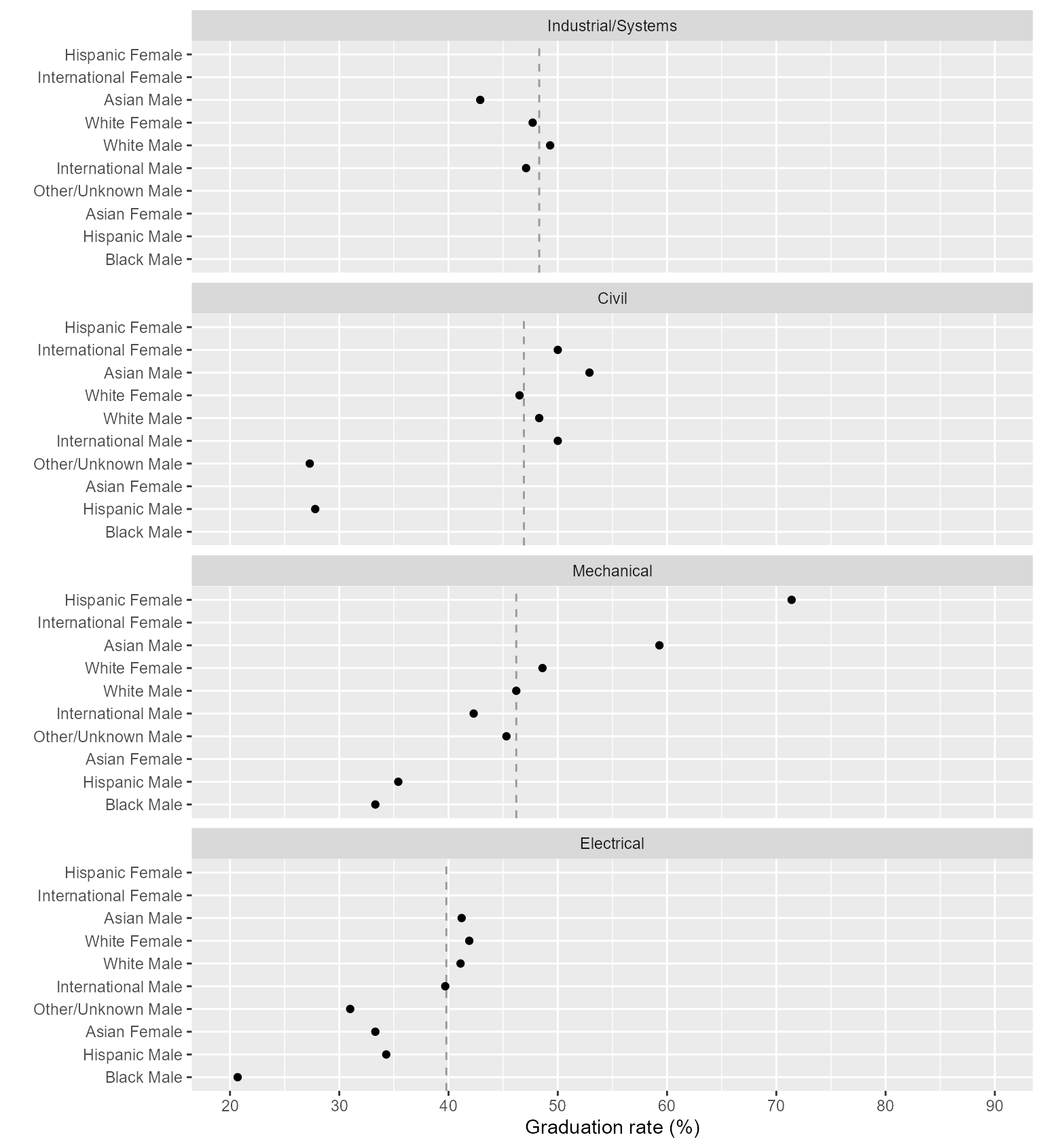

Figure 2: Graduation rates of four Engineering majors.

Table

Results table.   Code adapted from Multiway data and charts.

# Select variables and remove factors
display_table <- copy(DT)
display_table <- display_table[, .(program, people, rate)]
display_table[, people := as.character(people)]
display_table[, program := as.character(program)]

# Construct table
display_table <- dcast(display_table, people ~ program, value.var = "rate")
setnames(display_table,
  old = c("people"),
  new = c("People"),
  skip_absent = TRUE
)
display_table
#>                   People Civil Electrical Industrial/Systems Mechanical
#>  1:         Asian Female    NA       33.3                 NA         NA
#>  2:           Asian Male  52.9       41.2               42.9       59.3
#>  3:           Black Male    NA       20.7                 NA       33.3
#>  4: International Female  50.0         NA                 NA         NA
#>  5:   International Male  50.0       39.7               47.1       42.3
#>  6:        Latine Female    NA         NA                 NA       71.4
#>  7:          Latine Male  27.8       34.3                 NA       35.4
#>  8:   Other/Unknown Male  27.3       31.0                 NA       45.3
#>  9:         White Female  46.5       41.9               47.7       48.6
#> 10:           White Male  48.3       41.1               49.3       46.2

(Optional) Format the table nearer to publication quality. Here I use kableExtra package.

display_table |>
  kableExtra::kbl(align = "lrrrr", caption = "Table 2: Graduation rates (%) of four Engineering majors.") |>
  kableExtra::kable_paper(lightable_options = "basic", full_width = TRUE) |>
  kableExtra::row_spec(0, background = "#c7eae5") |>
  kableExtra::column_spec(1:5, color = "black", background = "white")

Table 2: Graduation rates (%) of four Engineering majors.

People	Civil	Electrical	Industrial/Systems	Mechanical
Asian Female	NA	33.3	NA	NA
Asian Male	52.9	41.2	42.9	59.3
Black Male	NA	20.7	NA	33.3
International Female	50.0	NA	NA	NA
International Male	50.0	39.7	47.1	42.3
Latine Female	NA	NA	NA	71.4
Latine Male	27.8	34.3	NA	35.4
Other/Unknown Male	27.3	31.0	NA	45.3
White Female	46.5	41.9	47.7	48.6
White Male	48.3	41.1	49.3	46.2

A value of NA indicates a group removed because the number of graduates was below the threshold set to preserve anonymity. As noted earlier, these are largely an artifact of applying these groupings to practice data.

References

Cook, Bryan, and Terry W. Hartle. 2011. “Why graduation rates matter—and why they don’t.” The Presidency Magazine, no. Spring/Summer 2011.

NCES-IPEDS. 2020. IPEDS Survey Methodology. National Center for Education Statistics; [Online; accessed 2020-07-29]. https://nces.ed.gov/ipeds/ReportYourData/IpedsSurveyMethodology.