Stickiness

Stickiness is a more-inclusive alternative to graduation rate as a measure of a program’s success in attracting, keeping, and graduating their undergraduates. All students excluded by a conventional graduation rate metric–including migrators—are included in the stickiness metric (Ohland et al. 2012).

This vignette in the MIDFIELD workflow.

1. Planning
   
2. Initial processing
   
3. Blocs
   
4. Groupings
   
5. Metrics
   • Graduation rate
     
   • Stickiness
     
6. Displays

Definitions

stickiness

Stickiness \((S)\) is the ratio of the number of graduates of a program \((N_g)\) to the number ever enrolled in the program \((N_e)\). \[ S = \frac{N_g}{N_e} \]

bloc

A grouping of student-level data dealt with as a unit, for example, starters, students ever-enrolled, graduates, transfer students, traditional and non-traditional students, migrators, etc.

ever-enrolled

Bloc of students whose term records include a specified program in at least one term.

graduates

Bloc of all graduates (timely completers) from a program, without regard to their starting programs.

timely completion criterion

Completing a program in no more than a specified span of years, in many cases, within 6 years after admission (150% of the “normal” 4-year span), or possibly less for some transfer students.

migrators

Bloc of students who leave one program to enroll in another. Also called switchers.

A more inclusive metric

Stickiness, in comparison to graduation rate, has these characteristics:

• Includes migrators, where graduation rate does not.

• Is based on the bloc of ever enrolled rather than starters, so there is no need for FYE proxies.

• Counts all graduates (timely completers) in a program, eliminating the need to filter graduates based on their starting program.

• Like the MIDFIELD definition of graduation rate (in contrast to the IPEDS definition), includes students who attend college part-time, who transfer between institutions, and who start in any term.

As they pertain to the stickiness metric, relationships among starters, migrators, and graduates (timely completers) of a given program P are illustrated in Figure 1.

• The interior rectangle represents the stickiness numerator \((N_g)\), the set of graduates (timely completers) of program P.

• The overall rectangle represents the stickiness denominator \((N_e)\), the set of students ever enrolled in program P.

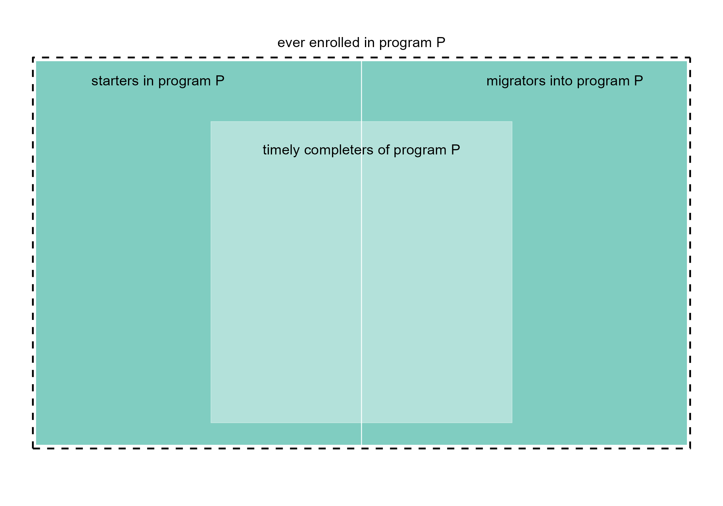
Figure 1. Stickiness metric. Starters, migrators, and timely completers.

Method

Demonstrating the following elements of a MIDFIELD workflow.

1. Planning.   The metric is stickiness. Required blocs are ever-enrolled and graduates. Grouping variables are program, race/ethnicity, and sex. Programs are the four Engineering programs used throughout.

2. Initial processing.   Filter the student-level records for data sufficiency and degree-seeking.

3. Blocs.   Gather ever enrolled, filter by program. Gather graduates, filter by program.

4. Groupings.   Add grouping variables.

5. Metrics   Summarize by grouping variables and compute stickiness.

6. Displays   Create multiway chart and results table.

Reminder.   midfielddata datasets are for practice, not research.

Load data

Start.   If you are writing your own script to follow along, we use these packages in this article:

library(midfieldr)
library(midfielddata)
library(data.table)
library(ggplot2)

Load.   Practice datasets. View data dictionaries via ?student, ?term, ?degree.

# Load practice data
data(student, term, degree)

Loads with midfieldr.   Prepared data. View data dictionary via ?study_programs, ?baseline_mcid.

• study_programs (derived in Programs).

• baseline_mcid (derived in Blocs).

Initial processing

Select (optional).   Reduce the number of columns. Code reproduced from Getting started.

# Optional. Copy of source files with all variables
source_student <- copy(student)
source_term <- copy(term)
source_degree <- copy(degree)

# Optional. Select variables required by midfieldr functions
student <- select_required(source_student)
term <- select_required(source_term)
degree <- select_required(source_degree)

Initialize.   From term and student, construct a data frame of student IDs filtered for data sufficiency and degree seeking as described in Blocs.

# Working data frame
DT <- copy(baseline_mcid)

Ever enrolled

Ever enrolled.   The summary code chunk from Blocs.

# Ever-enrolled bloc
DT <- term[DT, .(mcid, cip6), on = c("mcid")]
DT <- unique(DT)

# Filter by program
DT <- study_programs[DT, on = c("cip6"), nomatch = NULL]
DT[, cip6 := NULL]
DT <- unique(DT)
DT
#>       program           mcid
#>    1:      EE MCID3111142965
#>    2:      EE MCID3111145102
#>    3:      EE MCID3111146537
#>   ---                       
#> 5651:      ME MCID3112641399
#> 5652:      ME MCID3112641535
#> 5653:      ME MCID3112698681

Copy.   To prepare for joining with graduates.

# Prepare for joining
setcolorder(DT, c("mcid"))
ever_enrolled <- copy(DT)
ever_enrolled
#>                 mcid program
#>    1: MCID3111142965      EE
#>    2: MCID3111145102      EE
#>    3: MCID3111146537      EE
#>   ---                       
#> 5651: MCID3112641399      ME
#> 5652: MCID3112641535      ME
#> 5653: MCID3112698681      ME

Graduates

Initialize.   The data frame of baseline IDs is the intake for this section.

# Working data frame
DT <- copy(baseline_mcid)

Graduates   The summary code chunk from Graduates

# Gather graduates and their degree CIPs
DT <- add_timely_term(DT, term)
DT <- add_completion_status(DT, degree)
DT <- DT[completion_status == "timely"]
DT <- degree[DT, .(mcid, term_degree, cip6), on = c("mcid")]

# Filter by program and first-degree terms only
DT <- study_programs[DT, on = c("cip6"), nomatch = NULL]
DT <- DT[, .SD[which.min(term_degree)], by = "mcid"]
DT[, c("cip6", "term_degree") := NULL]
DT <- unique(DT)
DT
#>                 mcid program
#>    1: MCID3111142965      EE
#>    2: MCID3111145102      EE
#>    3: MCID3111146537      EE
#>   ---                       
#> 3262: MCID3112618976      ME
#> 3263: MCID3112619484      EE
#> 3264: MCID3112641535      ME

Copy.   To prepare for joining with ever enrolled

# Prepare for joining
setcolorder(DT, c("mcid"))
graduates <- copy(DT)
graduates
#>                 mcid program
#>    1: MCID3111142965      EE
#>    2: MCID3111145102      EE
#>    3: MCID3111146537      EE
#>   ---                       
#> 3262: MCID3112618976      ME
#> 3263: MCID3112619484      EE
#> 3264: MCID3112641535      ME

Groupings

One of our grouping variables (program) is already included in the data frames. The next grouping variable is bloc to distinguish starters from graduates when the two data frames are combined.

Add a variable.   Label ever enrolled and graduates.

# For grouping by bloc
ever_enrolled[, bloc := "ever_enrolled"]
graduates[, bloc := "graduates"]

Join.   Combine the two blocs to prepare for summarizing. A graduate has two observations in these data: one as ever enrolled and one as a graduate.

# Prepare for summarizing
DT <- rbindlist(list(ever_enrolled, graduates))
DT
#>                 mcid program          bloc
#>    1: MCID3111142965      EE ever_enrolled
#>    2: MCID3111145102      EE ever_enrolled
#>    3: MCID3111146537      EE ever_enrolled
#>   ---                                     
#> 8915: MCID3112618976      ME     graduates
#> 8916: MCID3112619484      EE     graduates
#> 8917: MCID3112641535      ME     graduates

Add variables.   Demographics from Groupings

# Join race/ethnicity and sex
cols_we_want <- student[, .(mcid, race, sex)]
DT <- cols_we_want[DT, on = c("mcid")]
DT
#>                 mcid          race    sex program          bloc
#>    1: MCID3111142965 International   Male      EE ever_enrolled
#>    2: MCID3111145102         White   Male      EE ever_enrolled
#>    3: MCID3111146537         Asian Female      EE ever_enrolled
#>   ---                                                          
#> 8915: MCID3112618976         White   Male      ME     graduates
#> 8916: MCID3112619484         White   Male      EE     graduates
#> 8917: MCID3112641535         White   Male      ME     graduates

Verify prepared data.   study_observations, included with midfieldr, contains the case study information developed above. Here we verify that the two data frames have the same content.

# Demonstrate equivalence
same_content(DT, study_observations)
#> [1] TRUE

Note.   MIDFIELD research findings are regularly grouped by program, race/ethnicity, and sex. However, applied to the practice data these groupings produce several groups with totals below the threshold we impose to preserve anonymity, introducing a number of NA values in the resulting charts and tables. These NAs are largely an artifact of applying these groupings to practice data.

Stickiness

Summarize.   Count the numbers of observations for each combination of the grouping variables.

# Count observations by group
grouping_variables <- c("bloc", "program", "sex", "race")
DT <- DT[, .N, by = grouping_variables]
setorderv(DT, grouping_variables)
DT
#>              bloc program    sex            race   N
#>  1: ever_enrolled      CE Female           Asian  15
#>  2: ever_enrolled      CE Female           Black   4
#>  3: ever_enrolled      CE Female   International  23
#> ---                                                 
#> 96:     graduates      ME   Male Native American   1
#> 97:     graduates      ME   Male   Other/Unknown  41
#> 98:     graduates      ME   Male           White 953

Reshape.   Transform to row-record form to set up the stickiness metric calculation. Transform the N column into two columns, one for ever-enrolled and one for graduates.

# Prepare to compute metric
DT <- dcast(DT, program + sex + race ~ bloc, value.var = "N", fill = 0)
DT
#>     program    sex            race ever_enrolled graduates
#>  1:      CE Female           Asian            15        10
#>  2:      CE Female           Black             4         1
#>  3:      CE Female   International            23        13
#> ---                                                       
#> 48:      ME   Male Native American             5         1
#> 49:      ME   Male   Other/Unknown            80        41
#> 50:      ME   Male           White          1596       953

Create a variable.   Compute the metric.

# Compute metric
DT[, stickiness := round(100 * graduates / ever_enrolled, 1)]
DT
#>     program    sex            race ever_enrolled graduates stickiness
#>  1:      CE Female           Asian            15        10       66.7
#>  2:      CE Female           Black             4         1       25.0
#>  3:      CE Female   International            23        13       56.5
#> ---                                                                  
#> 48:      ME   Male Native American             5         1       20.0
#> 49:      ME   Male   Other/Unknown            80        41       51.2
#> 50:      ME   Male           White          1596       953       59.7

Verify prepared data.   study_results, included with midfieldr, contains the case study information developed above. Here we verify that the two data frames have the same content.

# Demonstrate equivalence
same_content(DT, study_results)
#> [1] TRUE

Prepare for dissemination

Filter.   To preserve the anonymity of the people involved, we remove observations with fewer than N_threshold graduates. With the research data, we typically set this threshold to 10; with the practice data, we demonstrate the procedure using a threshold of 5.

# Preserve anonymity
N_threshold <- 5 # 10 for research data
DT <- DT[graduates >= N_threshold]
DT
#>     program    sex          race ever_enrolled graduates stickiness
#>  1:      CE Female         Asian            15        10       66.7
#>  2:      CE Female International            23        13       56.5
#>  3:      CE Female        Latine            13         6       46.2
#> ---                                                                
#> 33:      ME   Male        Latine            79        42       53.2
#> 34:      ME   Male Other/Unknown            80        41       51.2
#> 35:      ME   Male         White          1596       953       59.7

Recode.   Readers can more readily interpret our charts and tables if the programs are unabbreviated.

# Recode values for chart and table readability
DT[, program := fcase(
  program %like% "CE", "Civil",
  program %like% "EE", "Electrical",
  program %like% "ME", "Mechanical",
  program %like% "ISE", "Industrial/Systems"
)]
DT
#>        program    sex          race ever_enrolled graduates stickiness
#>  1:      Civil Female         Asian            15        10       66.7
#>  2:      Civil Female International            23        13       56.5
#>  3:      Civil Female        Latine            13         6       46.2
#> ---                                                                   
#> 33: Mechanical   Male        Latine            79        42       53.2
#> 34: Mechanical   Male Other/Unknown            80        41       51.2
#> 35: Mechanical   Male         White          1596       953       59.7

Add a variable.   We combine race/ethnicity and sex to create a combined grouping variable.

# Create a combined category
DT[, people := paste(race, sex)]
DT[, `:=`(race = NULL, sex = NULL)]
setcolorder(DT, c("program", "people"))
DT
#>        program               people ever_enrolled graduates stickiness
#>  1:      Civil         Asian Female            15        10       66.7
#>  2:      Civil International Female            23        13       56.5
#>  3:      Civil        Latine Female            13         6       46.2
#> ---                                                                   
#> 33: Mechanical          Latine Male            79        42       53.2
#> 34: Mechanical   Other/Unknown Male            80        41       51.2
#> 35: Mechanical           White Male          1596       953       59.7

Chart

Order factors.   Order the levels of the categories. Code adapted from Multiway data and charts.

# Order the categories
DT <- order_multiway(DT,
  quantity   = "stickiness",
  categories = c("program", "people"),
  method     = "percent",
  ratio_of   = c("graduates", "ever_enrolled")
)
DT
#>        program               people graduates ever_enrolled stickiness
#>  1:      Civil         Asian Female        10            15       66.7
#>  2:      Civil International Female        13            23       56.5
#>  3:      Civil        Latine Female         6            13       46.2
#> ---                                                                   
#> 33: Mechanical          Latine Male        42            79       53.2
#> 34: Mechanical   Other/Unknown Male        41            80       51.2
#> 35: Mechanical           White Male       953          1596       59.7
#>     program_stickiness people_stickiness
#>  1:               62.4              62.7
#>  2:               62.4              47.1
#>  3:               62.4              56.0
#> ---                                     
#> 33:               59.0              47.4
#> 34:               59.0              45.6
#> 35:               59.0              59.3

Multiway chart.   Code adapted from Multiway data and charts.

The vertical reference line is the aggregate stickiness of the program, independent of race/ethnicity and sex. A missing data marker or missing group indicates the number of graduates was below the threshold set to preserve anonymity—largely an artifact of applying these groupings to practice data.

ggplot(DT, aes(x = stickiness, y = people)) +
  facet_wrap(vars(program), ncol = 1, as.table = FALSE) +
  geom_vline(aes(xintercept = program_stickiness), linetype = 2, color = "gray60") +
  geom_point() +
  labs(x = "Stickiness (%)", y = "") +
  scale_x_continuous(limits = c(20, 90), breaks = seq(0, 100, 10))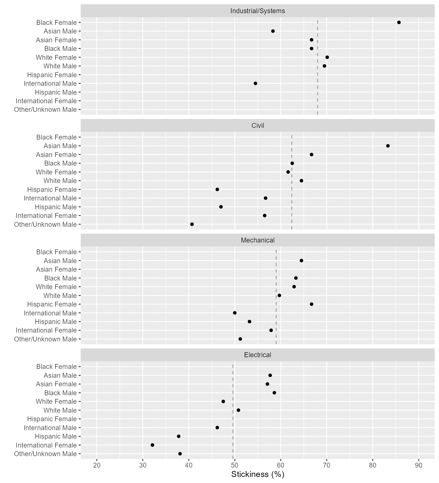

Figure 2: Stickiness of four Engineering majors.

Table

Results table.   Code adapted from Multiway data and charts.

# Select variables and remove factors
display_table <- copy(DT)
display_table <- display_table[, .(program, people, stickiness)]
display_table[, people := as.character(people)]
display_table[, program := as.character(program)]

# Construct table
display_table <- dcast(display_table, people ~ program, value.var = "stickiness")
setnames(display_table,
  old = c("people"),
  new = c("People"),
  skip_absent = TRUE
)
display_table
#>                 People Civil Electrical Industrial/Systems Mechanical
#>  1:       Asian Female  66.7       57.1               66.7         NA
#>  2:         Asian Male  83.3       57.7               58.3       64.5
#>  3:       Black Female    NA         NA               85.7         NA
#> ---                                                                  
#>  9: Other/Unknown Male  40.7       38.1                 NA       51.2
#> 10:       White Female  61.6       47.5               70.1       62.9
#> 11:         White Male  64.5       50.8               69.5       59.7

(Optional) Format the table nearer to publication quality. Here I use kableExtra package.

display_table |>
  kableExtra::kbl(align = "lrrrr", caption = "Table 1: Stickiness (%) of four Engineering majors.") |>
  kableExtra::kable_paper(lightable_options = "basic", full_width = TRUE) |>
  kableExtra::row_spec(0, background = "#c7eae5") |>
  kableExtra::column_spec(1:5, color = "black", background = "white")

Table 1: Stickiness (%) of four Engineering majors.

People	Civil	Electrical	Industrial/Systems	Mechanical
Asian Female	66.7	57.1	66.7	NA
Asian Male	83.3	57.7	58.3	64.5
Black Female	NA	NA	85.7	NA
Black Male	62.5	58.6	66.7	63.3
International Female	56.5	32.1	NA	57.9
International Male	56.7	46.2	54.5	50.0
Latine Female	46.2	NA	NA	66.7
Latine Male	47.0	37.8	NA	53.2
Other/Unknown Male	40.7	38.1	NA	51.2
White Female	61.6	47.5	70.1	62.9
White Male	64.5	50.8	69.5	59.7

A value of NA indicates a group removed because the number of graduates was below the threshold set to preserve anonymity. As noted earlier, these are largely an artifact of applying these groupings to practice data.

References

Ohland, Matthew, Marisa Orr, Richard Layton, Susan Lord, and Russell Long. 2012. “Introducing stickiness as a versatile metric of engineering persistence.” In Proceedings of the Frontiers in Education Conference, 1–5. DOI 10.1109/FIE.2012.6462214.