Case study using dplyr • midfieldr

In this study we present the same case as in the Case study article, but translated to use the syntax of the dplyr package and friends.

The study is concise, emphasizing process over details. (Terminology and functions are described in detail in subsequent articles.) Here we emphasize how we work with longitudinal data and how midfieldr supports that process.

Description

We define the parameters of our case study as follows:

Data. Program CIP codes from midfieldr cip. Student records from midfielddata student, term, and degree.

Metric. Program stickiness: the ratio \small (S) of the number of graduates of a program \small (N_\textrm{grad}) to the number ever enrolled in the program \small (N_\textrm{ever}), including part-time students, migrators, transfers, and students admitted in any term (Ohland et al. 2012).

\small S = \frac{\small N_\textrm{grad}}{\small N_\textrm{ever}} = \frac{\small\mathrm{number\ of\ graduates\ of\ a\ program}}{\small\mathrm{number\ ever\ enrolled\ in\ the\ program}}

Programs. Civil, Electrical, Industrial/Systems, and Mechanical Engineering.

Records. Exclude records later than a student’s first degree term; filter for data sufficiency and degree seeking; no exclusions due to part-time status, transfer status, admission term, or starting program.

Population. The set of unique IDs from the above records.

Blocs. Students ever enrolled in the programs and timely graduates of the programs are required by the metric.

Groupings. We select program, race/ethnicity, and sex for grouping and summarizing.

Outcome. To calculate the metric, we construct a data frame with columns for each grouping variable (program, race/ethnicity, and sex) and the counts by group \small N_\textrm{grad} and \small N_\textrm{ever}.

Dissemination. Exclude groupings too small to preserve anonymity. Edit column names to suit the audience. Condition/transform data as needed for tables or charts.

If you are writing your own script to follow along, we use these packages in this article:

library(midfieldr)
library(midfielddata)
library(dplyr)
library(tidyr)
library(stringr)

Programs

One can start an analysis with program data or with student record data—the choice is arbitrary. We start with programs and set the results aside until needed when constructing our blocs. Our goal in this section is to search the CIP data table for the 6-digit codes for our programs. The cip dataset loads with midfieldr.

Search for program codes

The cip dataset loads with midfieldr. For compatibility with the dplyr syntax, we covert it to a tibble.

cip <- as_tibble(cip)

Unless you already know your program CIP codes, finding them entails some trial and error.

filter_cip_rows() searches cip for string patterns. Searching for “civil engineering” yields programs in Engineering that we want and some in Engineering Technology that we do not.

filter_cip_rows(cip, "civil engineering")
#> # A tibble: 8 × 6
#>   cip6name                                       cip6  
#>   <chr>                                          <chr> 
#> 1 Civil Engineering, General                     140801
#> 2 Geotechnical Engineering                       140802
#> 3 Structural Engineering                         140803
#> 4 Transportation and Highway Engineering         140804
#> 5 Water Resources Engineering                    140805
#> 6 Civil Engineering, Other                       140899
#> 7 Civil Engineering Technology, Technician       150201
#> 8 Civil Drafting and Civil Engineering CAD, CADD 151304
#>   cip4name                                               cip4 
#>   <chr>                                                  <chr>
#> 1 Civil Engineering                                      1408 
#> 2 Civil Engineering                                      1408 
#> 3 Civil Engineering                                      1408 
#> 4 Civil Engineering                                      1408 
#> 5 Civil Engineering                                      1408 
#> 6 Civil Engineering                                      1408 
#> 7 Civil Engineering Technologies, Technicians            1502 
#> 8 Drafting, Design Engineering Technologies, Technicians 1513 
#>   cip2name               cip2 
#>   <chr>                  <chr>
#> 1 Engineering            14   
#> 2 Engineering            14   
#> 3 Engineering            14   
#> 4 Engineering            14   
#> 5 Engineering            14   
#> 6 Engineering            14   
#> 7 Engineering Technology 15   
#> 8 Engineering Technology 15

These results suggest that Engineering has the 2-digit code “14” and that Civil Engineering has the 4-digit code “1408”. We can extract Civil Engineering alone by searching cip for lines that start with “1408”, yielding six 6-digit codes. Regular expressions such as “^1408” are accepted.

cip |>
  filter_cip_rows("^1408")
#> # A tibble: 6 × 6
#>   cip6name                               cip6   cip4name          cip4 
#>   <chr>                                  <chr>  <chr>             <chr>
#> 1 Civil Engineering, General             140801 Civil Engineering 1408 
#> 2 Geotechnical Engineering               140802 Civil Engineering 1408 
#> 3 Structural Engineering                 140803 Civil Engineering 1408 
#> 4 Transportation and Highway Engineering 140804 Civil Engineering 1408 
#> 5 Water Resources Engineering            140805 Civil Engineering 1408 
#> 6 Civil Engineering, Other               140899 Civil Engineering 1408 
#>   cip2name    cip2 
#>   <chr>       <chr>
#> 1 Engineering 14   
#> 2 Engineering 14   
#> 3 Engineering 14   
#> 4 Engineering 14   
#> 5 Engineering 14   
#> 6 Engineering 14

Knowing the 2-digit code for Engineering programs, our next search is for lines that start with “14”. The result is an Engineering subset of cip with 54 rows.

cip |>
  filter_cip_rows("^14")
#> # A tibble: 54 × 6
#>   cip6name                                                     cip6  
#>   <chr>                                                        <chr> 
#> 1 Engineering, General                                         140101
#> 2 Pre-Engineering                                              140102
#> 3 Aerospace, Aeronautical and Astronautical, Space Engineering 140201
#> 4 Agricultural, Biological Engineering and Bioengineering      140301
#> 5 Architectural Engineering                                    140401
#>   cip4name                                                cip4  cip2name   
#>   <chr>                                                   <chr> <chr>      
#> 1 Engineering, General                                    1401  Engineering
#> 2 Engineering, General                                    1401  Engineering
#> 3 Aerospace, Aeronautical and Astronautical Engineering   1402  Engineering
#> 4 Agricultural, Biological Engineering and Bioengineering 1403  Engineering
#> 5 Architectural Engineering                               1404  Engineering
#>   cip2 
#>   <chr>
#> 1 14   
#> 2 14   
#> 3 14   
#> 4 14   
#> 5 14   
#> # ℹ 49 more rows

Next, to search this result for Electrical Engineering, we assign engr_cip to the cip argument, yielding four 6-digit codes.

cip |>
  filter_cip_rows("^14") |>
  filter_cip_rows("electrical")
#> # A tibble: 4 × 6
#>   cip6name                                                      cip6  
#>   <chr>                                                         <chr> 
#> 1 Electrical, Electronics and Communications Engineering        141001
#> 2 Laser and Optical Engineering                                 141003
#> 3 Telecommunications Engineering                                141004
#> 4 Electrical, Electronics and Communications Engineering, Other 141099
#>   cip4name                                               cip4  cip2name    cip2 
#>   <chr>                                                  <chr> <chr>       <chr>
#> 1 Electrical, Electronics and Communications Engineering 1410  Engineering 14   
#> 2 Electrical, Electronics and Communications Engineering 1410  Engineering 14   
#> 3 Electrical, Electronics and Communications Engineering 1410  Engineering 14   
#> 4 Electrical, Electronics and Communications Engineering 1410  Engineering 14

Continuing in a similar fashion, we find that our programs have the following 4-digit codes:

Civil Engineering 1408
Electrical Engineering 1410
Mechanical Engineering 1419
Industrial/Systems Engineering 1427, 1435, 1436, and 1437.

Construct the programs table

To collect all our 6-digit codes, we create a search string of the desired 4-digit codes. We drop all columns except the 6-digit names and 6-digit codes.

codes_we_want <- c("^1408", "^1410", "^1419", "^1427", "^1435", "^1436", "^1437")
programs <- cip |>
  filter_cip_rows(codes_we_want) |>
  select(cip6name, cip6)

programs
#> # A tibble: 15 × 2
#>   cip6name                               cip6  
#>   <chr>                                  <chr> 
#> 1 Civil Engineering, General             140801
#> 2 Geotechnical Engineering               140802
#> 3 Structural Engineering                 140803
#> 4 Transportation and Highway Engineering 140804
#> 5 Water Resources Engineering            140805
#> # ℹ 10 more rows

The program names in cip are usually too long for effective use—user-defined names are nearly always required. So we add a program variable with values “CE” (Civil Engineering), “EE” (electrical), “ME” (Mechanical), and “ISE” (Industrial-Systems Engineering). We also abbreviate a couple of terms for a slightly more compact display.

programs <- programs |>
  mutate(program = case_when(
    grepl("^1408", cip6) ~ "CE",
    grepl("^1410", cip6) ~ "EE",
    grepl("^1419", cip6) ~ "ME",
    grepl("^1427|^1435|^1436|^1437", cip6) ~ "ISE"
  )) |>
  mutate(across(cip6name, \(x) str_replace(x, "Engineering", "Engng"))) |>
  mutate(across(cip6name, \(x) str_replace(x, "Communication", "Commn")))

programs
#> # A tibble: 15 × 3
#>   cip6name                         cip6   program
#>   <chr>                            <chr>  <chr>  
#> 1 Civil Engng, General             140801 CE     
#> 2 Geotechnical Engng               140802 CE     
#> 3 Structural Engng                 140803 CE     
#> 4 Transportation and Highway Engng 140804 CE     
#> 5 Water Resources Engng            140805 CE     
#> # ℹ 10 more rows

Our programs data frame is complete: 15 six-digit codes are encoded using 4 program labels. This data frame can sit in memory (or written to file) until we’re ready to filter the blocs by program, joining data frames by matching on the cip6 variable.

Records

For this study we load three of the midfielddata data tables. We convert these data frames to tibbles as well.

data(student, term, degree)

student <- as_tibble(student)
term <- as_tibble(term)
degree <- as_tibble(degree)

We usually copy the source data, giving them new names (and new locations in memory), to keep them intact while we use the original names — student, term, and degree — to do our work. Unlike when using data.table, tibbles do not update by reference.

student_source <- student
term_source <- term
degree_source <- degree

The working data frames student, term, and degree should always be present in our computing environment so we can take advantage of midfieldr default argument values. For example, add_term_cluster() accesses the degree table to do its work. If degree is in the environment, the following lines yield the same results:

# not run
add_term_cluster(term, midfield_degree = degree)
add_term_cluster(term, degree)
add_term_cluster(term)

In this article, we use the latter form.

Select basic columns

Optional, but convenient for viewing data frames at intermediate stages. We reduce the number of columns to those required by other midfieldr functions plus the key or composite key variables of the data tables.

student <- select_record_cols(student, type = "s")
term <- select_record_cols(term, "t")
degree <- select_record_cols(degree, "d")

look_at() is a midfieldr convenience function that wraps base::str().

look_at(student)
#> tibble [97,555 × 3] (S3: tbl_df/tbl/data.frame)
#>  $ mcid: chr  "MCID3111142225" "MCID3111142283" "MCID3111142290" "MCID3111142"..
#>  $ race: chr  "Asian" "Asian" "Asian" "Asian" ...
#>  $ sex : chr  "Male" "Female" "Male" "Male" ...

look_at(term)
#> tibble [639,915 × 5] (S3: tbl_df/tbl/data.frame)
#>  $ mcid       : chr  "MCID3111142225" "MCID3111142283" "MCID3111142283" "MCID"..
#>  $ term       : chr  "19881" "19881" "19883" "19885" ...
#>  $ cip6       : chr  "140901" "240102" "240102" "190601" ...
#>  $ institution: chr  "Institution B" "Institution J" "Institution J" "Institu"..
#>  $ level      : chr  "01 First-year" "01 First-year" "01 First-year" "01 Firs"..

look_at(degree)
#> tibble [49,665 × 3] (S3: tbl_df/tbl/data.frame)
#>  $ mcid       : chr  "MCID3111142225" "MCID3111142290" "MCID3111142294" "MCID"..
#>  $ term_degree: chr  "19881" "19921" "19903" "19921" ...
#>  $ cip6       : chr  "141001" "141001" "141001" "141001" ...

Exclude post-baccalaureate terms

We are not generally interested in terms beyond the first degree term, so we identify and exclude terms later than the first degree term. Multiple degrees earned in the first degree term are retained, but any courses, terms, or degrees after the first baccalaureate are excluded.

add_term_cluster() adds a column of labels indicating that a term belongs to one of three clusters: terms that are prior to, equal to, or subsequent to the student’s first degree term.

term <- add_term_cluster(term)
degree <- add_term_cluster(degree)

look_at(term)
#> tibble [639,915 × 7] (S3: tbl_df/tbl/data.frame)
#>  $ mcid             : chr  "MCID3111142225" "MCID3111142283" "MCID3111142283""..
#>  $ term             : chr  "19881" "19881" "19883" "19885" ...
#>  $ cip6             : chr  "140901" "240102" "240102" "190601" ...
#>  $ institution      : chr  "Institution B" "Institution J" "Institution J" "I"..
#>  $ level            : chr  "01 First-year" "01 First-year" "01 First-year" "0"..
#>  $ first_degree_term: chr  "19881" NA NA NA ...
#>  $ term_cluster     : chr  "first-degree" "pre-degree" "pre-degree" "pre-degr"..

look_at(degree)
#> tibble [49,665 × 5] (S3: tbl_df/tbl/data.frame)
#>  $ mcid             : chr  "MCID3111142225" "MCID3111142290" "MCID3111142294""..
#>  $ term_degree      : chr  "19881" "19921" "19903" "19921" ...
#>  $ cip6             : chr  "141001" "141001" "141001" "141001" ...
#>  $ first_degree_term: chr  "19881" "19921" "19903" "19921" ...
#>  $ term_cluster     : chr  "first-degree" "first-degree" "first-degree" "firs"..

To quickly assess the relative size of the three clusters, we count observations by the term_cluster variable.

term |>
  group_by(term_cluster) |>
  tally() |>
  arrange(desc(n))
#> # A tibble: 3 × 2
#>   term_cluster           n
#>   <chr>              <int>
#> 1 pre-degree        598477
#> 2 first-degree       34440
#> 3 post-first-degree   6998

degree |>
  group_by(term_cluster) |>
  tally() |>
  arrange(desc(n))
#> # A tibble: 2 × 2
#>   term_cluster          n
#>   <chr>             <int>
#> 1 first-degree      49618
#> 2 post-first-degree    47

We exclude the rows labeled “post-first-degree.” This step does not apply to the student table because it contains no term information.

term <- term |>
  filter(term_cluster != "post-first-degree")

degree <- degree |>
  filter(term_cluster != "post-first-degree")

We can drop the added columns by applying select_record_cols() again.

term <- select_record_cols(term, "t")
degree <- select_record_cols(degree, "d")

look_at(term)
#> tibble [632,917 × 5] (S3: tbl_df/tbl/data.frame)
#>  $ mcid       : chr  "MCID3111142225" "MCID3111142283" "MCID3111142283" "MCID"..
#>  $ term       : chr  "19881" "19881" "19883" "19885" ...
#>  $ cip6       : chr  "140901" "240102" "240102" "190601" ...
#>  $ institution: chr  "Institution B" "Institution J" "Institution J" "Institu"..
#>  $ level      : chr  "01 First-year" "01 First-year" "01 First-year" "01 Firs"..

look_at(degree)
#> tibble [49,618 × 3] (S3: tbl_df/tbl/data.frame)
#>  $ mcid       : chr  "MCID3111142225" "MCID3111142290" "MCID3111142294" "MCID"..
#>  $ term_degree: chr  "19881" "19921" "19903" "19921" ...
#>  $ cip6       : chr  "141001" "141001" "141001" "141001" ...

Filter for data sufficiency

The next few steps are easier to follow if we start with the unique IDs from our current term table as our draft population. We filter these IDs for data sufficiency and degree-seeking, then filter the records to retain those IDs only.

DT <- term |>
  select(mcid) |>
  unique()
DT
#> # A tibble: 97,536 × 1
#>   mcid          
#>   <chr>         
#> 1 MCID3111142225
#> 2 MCID3111142283
#> 3 MCID3111142290
#> 4 MCID3111142294
#> 5 MCID3111142299
#> # ℹ 97,531 more rows

The data sufficiency criterion limits student records to those for which available data are sufficient to credibly assess timely completion. To make that assessment, we need the last term in which a student’s degree completion would be considered timely—in many cases, 6 years after admission.

add_timely_term() adds a column of timely completion terms, encoded YYYYT.

DT <- add_timely_term(DT)
DT
#> # A tibble: 97,536 × 5
#>   mcid           term_i level_i       adj_span timely_term
#>   <chr>          <chr>  <chr>            <dbl> <chr>      
#> 1 MCID3111142225 19881  01 First-year        6 19933      
#> 2 MCID3111142283 19881  01 First-year        6 19933      
#> 3 MCID3111142290 19881  01 First-year        6 19933      
#> 4 MCID3111142294 19881  01 First-year        6 19933      
#> 5 MCID3111142299 19881  01 First-year        6 19933      
#> # ℹ 97,531 more rows

add_data_sufficiency() (which requires the timely_term column) adds a column of labels indicating that a student ID should be included (or excluded) because for that student, the institution’s data range satisfies (or does not satisfy) the data sufficiency criteria.

DT <- add_data_sufficiency(DT)
DT
#> # A tibble: 97,536 × 8
#>   mcid           level_i       adj_span timely_term term_i lower_limit
#>   <chr>          <chr>            <dbl> <chr>       <chr>  <chr>      
#> 1 MCID3111142225 01 First-year        6 19933       19881  19881      
#> 2 MCID3111142283 01 First-year        6 19933       19881  19881      
#> 3 MCID3111142290 01 First-year        6 19933       19881  19881      
#> 4 MCID3111142294 01 First-year        6 19933       19881  19881      
#> 5 MCID3111142299 01 First-year        6 19933       19881  19881      
#>   upper_limit data_sufficiency
#>   <chr>       <chr>           
#> 1 20181       exclude-lower   
#> 2 20096       exclude-lower   
#> 3 20096       exclude-lower   
#> 4 20096       exclude-lower   
#> 5 20096       exclude-lower   
#> # ℹ 97,531 more rows

Again, a quick assessment of the relative size of the three possible labels.

DT |>
  group_by(data_sufficiency) |>
  tally() |>
  arrange(desc(n))
#> # A tibble: 3 × 2
#>   data_sufficiency     n
#>   <chr>            <int>
#> 1 include          76865
#> 2 exclude-upper    17925
#> 3 exclude-lower     2746

We retain the rows labeled “include” for which we have sufficient data from the institution and retain the ID column only.

DT <- DT |>
  filter(data_sufficiency == "include") |>
  select(mcid)
DT
#> # A tibble: 76,865 × 1
#>   mcid          
#>   <chr>         
#> 1 MCID3111142689
#> 2 MCID3111142782
#> 3 MCID3111142881
#> 4 MCID3111142884
#> 5 MCID3111142893
#> # ℹ 76,860 more rows

Filter for degree seeking

We require all students in our study to be degree-seeking. By design, the student table contains only degree-seeking students. We inner-join the ID column from the student table, matching on mcid. In effect, the inner join filters our population to remove any non-degree-seeking students.

DT <- inner_join(DT, student, by = join_by(mcid)) |>
  select(mcid)
DT
#> # A tibble: 76,865 × 1
#>   mcid          
#>   <chr>         
#> 1 MCID3111142689
#> 2 MCID3111142782
#> 3 MCID3111142881
#> 4 MCID3111142884
#> 5 MCID3111142893
#> # ℹ 76,860 more rows

It happens that all students in this case are degree-seeking, so this step did not reduce the size of our population. (We include the step to illustrate our complete process.)

Finalize the records

The previous column of IDs is our baseline population.

population <- unique(DT)
population
#> # A tibble: 76,865 × 1
#>   mcid          
#>   <chr>         
#> 1 MCID3111142689
#> 2 MCID3111142782
#> 3 MCID3111142881
#> 4 MCID3111142884
#> 5 MCID3111142893
#> # ℹ 76,860 more rows

We now filter the records to retain only those observations associated with the IDs in our population data frame. We use inner joins between population and student, term, and degree to do so. Ensuring rows are unique yields the baseline records in their final configuration.

student <- inner_join(student, population, by = join_by(mcid)) |>
  unique()
term <- inner_join(term, population, by = join_by(mcid)) |>
  unique()
degree <- inner_join(degree, population, by = join_by(mcid)) |>
  unique()

These three data frames are our final set of records on which all further analysis is based. We’ve reduced the number of unique students from 97,555 in the original source data to 76,865 that have met our several constraints.

look_at(student)
#> tibble [76,865 × 3] (S3: tbl_df/tbl/data.frame)
#>  $ mcid: chr  "MCID3111142689" "MCID3111142782" "MCID3111142881" "MCID3111142"..
#>  $ race: chr  "Hispanic" "Hispanic" "International" "International" ...
#>  $ sex : chr  "Female" "Female" "Male" "Male" ...

look_at(term)
#> tibble [525,446 × 5] (S3: tbl_df/tbl/data.frame)
#>  $ mcid       : chr  "MCID3111142689" "MCID3111142782" "MCID3111142782" "MCID"..
#>  $ term       : chr  "19883" "19883" "19885" "19893" ...
#>  $ cip6       : chr  "090401" "260101" "260101" "260101" ...
#>  $ institution: chr  "Institution B" "Institution J" "Institution J" "Institu"..
#>  $ level      : chr  "01 First-year" "01 First-year" "02 Second-year" "02 Sec"..

look_at(degree)
#> tibble [43,847 × 3] (S3: tbl_df/tbl/data.frame)
#>  $ mcid       : chr  "MCID3111142689" "MCID3111142782" "MCID3111142881" "MCID"..
#>  $ term_degree: chr  "19913" "19903" "19894" "19901" ...
#>  $ cip6       : chr  "090401" "260101" "450601" "141001" ...

Blocs and groupings

The work up to this point is applicable to most studies. In summary, we have configured our:

programs 6-digit program codes, names, and custom labels
student, term, and degree records with post-baccalaureate terms removed and filtered for data sufficiency and degree seeking
population the unique IDs in these records

The next steps depend on the metric and the groupings we assigned at the beginning. The stickiness metric requires these blocs:

students with timely completion from the study programs
students ever enrolled in these programs

And we selected these groupings:

program
race/ethnicity
sex

We have a lot of flexibility in the order in which we construct our blocs and groupings, so what follows is only one of several effective solutions. Our approach here is to construct a bloc, filter by program, join the demographics, and repeat for the next bloc.

Timely graduates

We start with the baseline population. Like we did with the original source data files, we copy it to protect population from “by reference” changes.

DT <- population
DT
#> # A tibble: 76,865 × 1
#>   mcid          
#>   <chr>         
#> 1 MCID3111142689
#> 2 MCID3111142782
#> 3 MCID3111142881
#> 4 MCID3111142884
#> 5 MCID3111142893
#> # ℹ 76,860 more rows

Filter for timely completion

We want to retain timely graduates, so first we add the timely completion term (the same term we used for determining data sufficiency) to our population then apply the completion status function.

add_completion_status() adds a column of labels indicating that program completion was timely, late, or NA (for non-completers).

DT <- DT |>
  add_timely_term() |>
  add_completion_status()
DT
#> # A tibble: 76,865 × 7
#>   mcid           term_i level_i       adj_span timely_term term_degree
#>   <chr>          <chr>  <chr>            <dbl> <chr>       <chr>      
#> 1 MCID3111142689 19883  01 First-year        6 19941       19913      
#> 2 MCID3111142782 19883  01 First-year        6 19941       19903      
#> 3 MCID3111142881 19893  01 First-year        6 19951       19894      
#> 4 MCID3111142884 19883  01 First-year        6 19941       NA         
#> 5 MCID3111142893 19883  01 First-year        6 19941       NA         
#>   completion_status
#>   <chr>            
#> 1 timely           
#> 2 timely           
#> 3 timely           
#> 4 NA               
#> 5 NA               
#> # ℹ 76,860 more rows

Another brief assessment. Here we compare the relative size of the three possible status labels.

DT |>
  group_by(completion_status) |>
  tally() |>
  arrange(desc(n))
#> # A tibble: 3 × 2
#>   completion_status     n
#>   <chr>             <int>
#> 1 timely            40430
#> 2 NA                33089
#> 3 late               3346

We retain the rows labeled “timely” and the drop all the columns except the ID column.

DT <- DT |>
  filter(completion_status == "timely") |>
  select(mcid)
DT
#> # A tibble: 40,430 × 1
#>   mcid          
#>   <chr>         
#> 1 MCID3111142689
#> 2 MCID3111142782
#> 3 MCID3111142881
#> 4 MCID3111142965
#> 5 MCID3111143066
#> # ℹ 40,425 more rows

Filter by program

We left-join the CIP column from the degree table, matching on mcid. That we increase the number of rows indicates that some students have more than one degree in their first degree term.

degree_cols <- degree |>
  select(mcid, cip6)
DT <- left_join(DT, degree_cols, by = join_by(mcid))
DT
#> # A tibble: 40,490 × 2
#>   mcid           cip6  
#>   <chr>          <chr> 
#> 1 MCID3111142689 090401
#> 2 MCID3111142782 260101
#> 3 MCID3111142881 450601
#> 4 MCID3111142965 141001
#> 5 MCID3111143066 090401
#> # ℹ 40,485 more rows

Now we use an inner-join with our programs data frame, matching on cip6, to retain only those students who complete one of our study programs. We retain the program column and drop the cip6 column.

programs_cols <- programs |>
  select(cip6, program)
DT <- inner_join(DT, programs_cols, by = join_by(cip6)) |>
  select(-cip6)
DT
#> # A tibble: 3,263 × 2
#>   mcid           program
#>   <chr>          <chr>  
#> 1 MCID3111142965 EE     
#> 2 MCID3111145102 EE     
#> 3 MCID3111146537 EE     
#> 4 MCID3111146674 EE     
#> 5 MCID3111150194 ISE    
#> # ℹ 3,258 more rows

Another brief assessment. Here we compare the relative numbers of program graduates.

DT |>
  group_by(program) |>
  tally() |>
  arrange(desc(n))
#> # A tibble: 4 × 2
#>   program     n
#>   <chr>   <int>
#> 1 ME       1353
#> 2 CE        936
#> 3 EE        736
#> 4 ISE       238

Join demographics

To add columns for student demographics, we left-join selected columns from the student table, matching on mcid.

student_cols <- student |>
  select(mcid, race, sex)
DT <- left_join(DT, student_cols, by = join_by(mcid))
DT
#> # A tibble: 3,263 × 4
#>   mcid           program race          sex   
#>   <chr>          <chr>   <chr>         <chr> 
#> 1 MCID3111142965 EE      International Male  
#> 2 MCID3111145102 EE      White         Male  
#> 3 MCID3111146537 EE      Asian         Female
#> 4 MCID3111146674 EE      Asian         Male  
#> 5 MCID3111150194 ISE     Black         Male  
#> # ℹ 3,258 more rows

Bloc of timely graduates

This is the bloc of timely graduates required by our metric. We add a bloc variable with the value “grad” and ensure we have unique rows.

graduates <- DT |>
  mutate(bloc = "grad") |>
  unique()

graduates
#> # A tibble: 3,263 × 5
#>   mcid           program race          sex    bloc 
#>   <chr>          <chr>   <chr>         <chr>  <chr>
#> 1 MCID3111142965 EE      International Male   grad 
#> 2 MCID3111145102 EE      White         Male   grad 
#> 3 MCID3111146537 EE      Asian         Female grad 
#> 4 MCID3111146674 EE      Asian         Male   grad 
#> 5 MCID3111150194 ISE     Black         Male   grad 
#> # ℹ 3,258 more rows

Ever enrolled

Again we start with the baseline population.

DT <- population
DT
#> # A tibble: 76,865 × 1
#>   mcid          
#>   <chr>         
#> 1 MCID3111142689
#> 2 MCID3111142782
#> 3 MCID3111142881
#> 4 MCID3111142884
#> 5 MCID3111142893
#> # ℹ 76,860 more rows

Filter by program

We left-join the CIP column from the term table, matching on mcid.

term_cols <- term |>
  select(mcid, cip6) |>
  unique()
DT <- left_join(DT, term_cols, by = join_by(mcid))
DT
#> # A tibble: 126,168 × 2
#>   mcid           cip6  
#>   <chr>          <chr> 
#> 1 MCID3111142689 090401
#> 2 MCID3111142782 260101
#> 3 MCID3111142881 450601
#> 4 MCID3111142884 260406
#> 5 MCID3111142893 400801
#> # ℹ 126,163 more rows

We repeat the process we used earlier to inner-join our programs data frame, matching on cip6.

programs_cols <- programs |>
  select(cip6, program)
DT <- inner_join(DT, programs_cols, by = join_by(cip6)) |>
  select(-cip6)
DT
#> # A tibble: 5,583 × 2
#>   mcid           program
#>   <chr>          <chr>  
#> 1 MCID3111142965 EE     
#> 2 MCID3111145102 EE     
#> 3 MCID3111146537 EE     
#> 4 MCID3111146674 EE     
#> 5 MCID3111150194 ISE    
#> # ℹ 5,578 more rows

With the CIP code removed, we filter for unique rows. This is an important step because a student may switch CIP codes yet stay within a program as defined by our custom labels. We want to avoid counting that student as ever-enrolled more than once.

DT <- unique(DT)
DT
#> # A tibble: 5,583 × 2
#>   mcid           program
#>   <chr>          <chr>  
#> 1 MCID3111142965 EE     
#> 2 MCID3111145102 EE     
#> 3 MCID3111146537 EE     
#> 4 MCID3111146674 EE     
#> 5 MCID3111150194 ISE    
#> # ℹ 5,578 more rows

Another brief assessment. Here we compare the relative numbers of students ever enrolled in our programs.

DT |>
  group_by(program) |>
  tally() |>
  arrange(desc(n))
#> # A tibble: 4 × 2
#>   program     n
#>   <chr>   <int>
#> 1 ME       2289
#> 2 CE       1494
#> 3 EE       1464
#> 4 ISE       336

Join demographics

Again, we left-join selected columns from the student table, matching on mcid.

student_cols <- student |>
  select(mcid, race, sex)
DT <- left_join(DT, student_cols, by = join_by(mcid))
DT
#> # A tibble: 5,583 × 4
#>   mcid           program race          sex   
#>   <chr>          <chr>   <chr>         <chr> 
#> 1 MCID3111142965 EE      International Male  
#> 2 MCID3111145102 EE      White         Male  
#> 3 MCID3111146537 EE      Asian         Female
#> 4 MCID3111146674 EE      Asian         Male  
#> 5 MCID3111150194 ISE     Black         Male  
#> # ℹ 5,578 more rows

Bloc of ever-enrolled

This is the bloc of students ever enrolled in our programs required by our metric. We add a bloc variable with the value “ever” and ensure we have unique rows.

ever_enrolled <- DT |>
  mutate(bloc = "ever") |>
  unique()

ever_enrolled
#> # A tibble: 5,583 × 5
#>   mcid           program race          sex    bloc 
#>   <chr>          <chr>   <chr>         <chr>  <chr>
#> 1 MCID3111142965 EE      International Male   ever 
#> 2 MCID3111145102 EE      White         Male   ever 
#> 3 MCID3111146537 EE      Asian         Female ever 
#> 4 MCID3111146674 EE      Asian         Male   ever 
#> 5 MCID3111150194 ISE     Black         Male   ever 
#> # ℹ 5,578 more rows

Outcomes

Combining the two data frames (blocs) by rows, we obtain the data structure we need for grouping and summarizing.

DT <- bind_rows(graduates, ever_enrolled)
DT
#> # A tibble: 8,846 × 5
#>   mcid           program race          sex    bloc 
#>   <chr>          <chr>   <chr>         <chr>  <chr>
#> 1 MCID3111142965 EE      International Male   grad 
#> 2 MCID3111145102 EE      White         Male   grad 
#> 3 MCID3111146537 EE      Asian         Female grad 
#> 4 MCID3111146674 EE      Asian         Male   grad 
#> 5 MCID3111150194 ISE     Black         Male   grad 
#> # ℹ 8,841 more rows

Group and summarize

Count the numbers of observations for each combination of the grouping variables.

DT <- DT %>%
  count(bloc, program, race, sex, name = "N")
DT
#> # A tibble: 98 × 5
#>   bloc  program race     sex        N
#>   <chr> <chr>   <chr>    <chr>  <int>
#> 1 ever  CE      Asian    Female    14
#> 2 ever  CE      Asian    Male      30
#> 3 ever  CE      Black    Female     4
#> 4 ever  CE      Black    Male       8
#> 5 ever  CE      Hispanic Female    13
#> # ℹ 93 more rows

Reshape

Reshaping the data frame to calculate the metric.

Transform from block-record form to row-record form. The N column values are moved to two new columns, ever and grad, one for each bloc, leaving the grouping variables (program, race/ethnicity, and sex) in place. This operation is known by a number of different names, e.g., pivot, crosstab, unstack, spread, or widen (Mount and Zumel 2019). The result has the data structure we called out in our project description for calculating the metric.

DT <- DT |>
  pivot_wider(
    names_from = bloc,
    values_from = N,
    values_fill = 0
  )
DT
#> # A tibble: 50 × 5
#>   program race     sex     ever  grad
#>   <chr>   <chr>    <chr>  <int> <int>
#> 1 CE      Asian    Female    14    10
#> 2 CE      Asian    Male      30    25
#> 3 CE      Black    Female     4     1
#> 4 CE      Black    Male       8     5
#> 5 CE      Hispanic Female    13     6
#> # ℹ 45 more rows

Calculate the metric

Completes the initial analysis.

Stickiness is the ratio of the number of graduates to the number ever enrolled, expressed as a percentage. Stickiness is calculated for each combination of program, race/ethnicity, and sex.

DT <- DT |>
  mutate(stickiness = round(100 * grad / ever, 1))
DT
#> # A tibble: 50 × 6
#>   program race     sex     ever  grad stickiness
#>   <chr>   <chr>    <chr>  <int> <int>      <dbl>
#> 1 CE      Asian    Female    14    10       71.4
#> 2 CE      Asian    Male      30    25       83.3
#> 3 CE      Black    Female     4     1       25  
#> 4 CE      Black    Male       8     5       62.5
#> 5 CE      Hispanic Female    13     6       46.2
#> # ℹ 45 more rows

Dissemination

We take several additional steps before disseminating these results.

To preserve the anonymity of the people involved, we remove observations with \small N or fewer observations. When dealing with the full MIDFIELD research data, we typically use \small N = 10, but for these practice data we illustrate the procedure using \small N = 3.

DT <- DT |>
  filter(grad > 3)
DT
#> # A tibble: 37 × 6
#>   program race     sex     ever  grad stickiness
#>   <chr>   <chr>    <chr>  <int> <int>      <dbl>
#> 1 CE      Asian    Female    14    10       71.4
#> 2 CE      Asian    Male      30    25       83.3
#> 3 CE      Black    Male       8     5       62.5
#> 4 CE      Hispanic Female    13     6       46.2
#> 5 CE      Hispanic Male      66    31       47  
#> # ℹ 32 more rows

We have found it useful to report such data with a variable that combines race/ethnicity and sex.

DT <- DT |>
  mutate(people = paste(race, sex)) |>
  select(program, race, sex, people, everything())
DT
#> # A tibble: 37 × 7
#>   program race     sex    people           ever  grad stickiness
#>   <chr>   <chr>    <chr>  <chr>           <int> <int>      <dbl>
#> 1 CE      Asian    Female Asian Female       14    10       71.4
#> 2 CE      Asian    Male   Asian Male         30    25       83.3
#> 3 CE      Black    Male   Black Male          8     5       62.5
#> 4 CE      Hispanic Female Hispanic Female    13     6       46.2
#> 5 CE      Hispanic Male   Hispanic Male      66    31       47  
#> # ℹ 32 more rows

Readers can more readily interpret our charts and tables if the programs are unabbreviated.

DT <- DT |>
  mutate(program = case_when(
    program == "CE" ~ "Civil",
    program == "EE" ~ "Electrical",
    program == "ME" ~ "Mechanical",
    program == "ISE" ~ "Industrial"
  ))
DT
#> # A tibble: 37 × 7
#>   program race     sex    people           ever  grad stickiness
#>   <chr>   <chr>    <chr>  <chr>           <int> <int>      <dbl>
#> 1 Civil   Asian    Female Asian Female       14    10       71.4
#> 2 Civil   Asian    Male   Asian Male         30    25       83.3
#> 3 Civil   Black    Male   Black Male          8     5       62.5
#> 4 Civil   Hispanic Female Hispanic Female    13     6       46.2
#> 5 Civil   Hispanic Male   Hispanic Male      66    31       47  
#> # ℹ 32 more rows

Table

Omit columns that won’t appear in the table.

DT_table <- DT |>
  select(program, people, stickiness)
DT_table
#> # A tibble: 37 × 3
#>   program people          stickiness
#>   <chr>   <chr>                <dbl>
#> 1 Civil   Asian Female          71.4
#> 2 Civil   Asian Male            83.3
#> 3 Civil   Black Male            62.5
#> 4 Civil   Hispanic Female       46.2
#> 5 Civil   Hispanic Male         47  
#> # ℹ 32 more rows

Transform the data from block-records to row-records with one row per “people” category (race/ethnicity/sex grouping).

DT_table <- DT_table |>
  pivot_wider(
    names_from = program,
    values_from = stickiness,
    values_fill = NA
  ) |>
  arrange(people) |>
  rename(People = people)
DT_table
#> # A tibble: 12 × 5
#>   People          Civil Electrical Industrial Mechanical
#>   <chr>           <dbl>      <dbl>      <dbl>      <dbl>
#> 1 Asian Female     71.4       57.1       66.7       NA  
#> 2 Asian Male       83.3       58.2       66.7       64.5
#> 3 Black Female     NA         NA         85.7       NA  
#> 4 Black Male       62.5       58.6       66.7       65.5
#> 5 Hispanic Female  46.2       NA         NA         66.7
#> # ℹ 7 more rows

Format the table for publication.

library(gt)
DT_table |>
  gt() |>
  tab_caption("Table 1. Engineering program stickiness (%)") |>
  tab_options(table.font.size = "small") |>
  opt_stylize(style = 1, color = "gray") |>
  tab_style(
    style = list(cell_fill(color = "#c7eae5")),
    locations = cells_column_labels(columns = everything())
  )

Table 1. Engineering program stickiness (%)
People	Civil	Electrical	Industrial	Mechanical
Asian Female	71.4	57.1	66.7	NA
Asian Male	83.3	58.2	66.7	64.5
Black Female	NA	NA	85.7	NA
Black Male	62.5	58.6	66.7	65.5
Hispanic Female	46.2	NA	NA	66.7
Hispanic Male	47.0	38.6	66.7	53.8
International Female	56.5	33.3	NA	57.9
International Male	56.7	46.4	57.1	50.6
Other/Unknown Female	NA	NA	NA	50.0
Other/Unknown Male	40.7	40.0	NA	51.2
White Female	62.3	47.9	74.0	63.2
White Male	64.9	52.0	73.0	60.1

Chart

To use ggplot(), we want the data in its block-record form.

DT_chart <- DT
DT_chart
#> # A tibble: 37 × 7
#>   program race     sex    people           ever  grad stickiness
#>   <chr>   <chr>    <chr>  <chr>           <int> <int>      <dbl>
#> 1 Civil   Asian    Female Asian Female       14    10       71.4
#> 2 Civil   Asian    Male   Asian Male         30    25       83.3
#> 3 Civil   Black    Male   Black Male          8     5       62.5
#> 4 Civil   Hispanic Female Hispanic Female    13     6       46.2
#> 5 Civil   Hispanic Male   Hispanic Male      66    31       47  
#> # ℹ 32 more rows

With one quantitative variable (stickiness) for every combination of the levels of two categorical variables (program and people), these are multiway data (Cleveland 1993). How one orders the categorical variables is critical for visualizing effects.

order_multiway() converts the two categorical variables to ordered factors to support the ordering of rows and panels in the chart. The calculated stickiness values by group—which determine the ordering—are added in new columns.

DT_chart <- order_multiway(DT_chart,
  quantity = "stickiness",
  categories = c("program", "people"),
  method = "percent",
  ratio_of = c("grad", "ever")
)
DT_chart
#> # A tibble: 37 × 9
#>   program people           grad  ever stickiness race     sex   
#>   <fct>   <fct>           <dbl> <dbl>      <dbl> <chr>    <chr> 
#> 1 Civil   Asian Female       10    14       71.4 Asian    Female
#> 2 Civil   Asian Male         25    30       83.3 Asian    Male  
#> 3 Civil   Black Male          5     8       62.5 Black    Male  
#> 4 Civil   Hispanic Female     6    13       46.2 Hispanic Female
#> 5 Civil   Hispanic Male      31    66       47   Hispanic Male  
#>   program_stickiness people_stickiness
#>                <dbl>             <dbl>
#> 1               62.8              64  
#> 2               62.8              63.9
#> 3               62.8              62.7
#> 4               62.8              56  
#> 5               62.8              48.5
#> # ℹ 32 more rows

Format the chart for publication.

library(ggplot2)
ggplot(DT_chart, aes(x = stickiness, y = people)) +
  facet_wrap(vars(program),
    ncol = 1,
    as.table = FALSE
  ) +
  geom_vline(aes(xintercept = program_stickiness),
    linetype = 2,
    color = "gray60"
  ) +
  geom_point(size = 1.8) +
  labs(x = "Stickiness (%)", y = "") +
  theme_light(base_size = 10)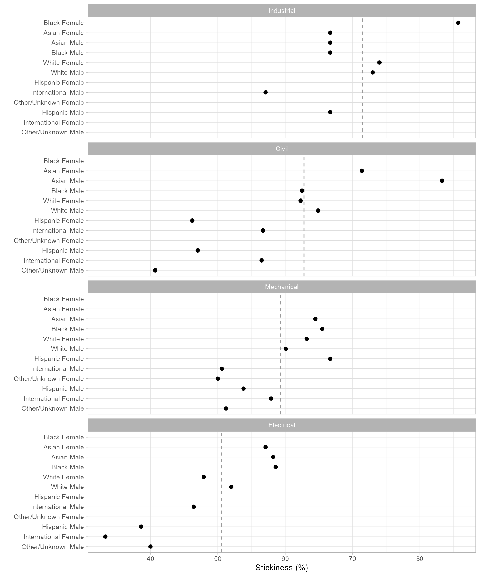

Figure 1: Program stickiness.

References

Cleveland, William S. 1993. Visualizing Data. Hobart Press.

Mount, John, and Nina Zumel. 2019. Coordinatized data: A fluid data specification. Win Vector LLC. http://winvector.github.io/FluidData/RowsAndColumns.html.

Ohland, Matthew, Marisa Orr, Richard Layton, Susan Lord, and Russell Long. 2012. “Introducing stickiness as a versatile metric of engineering persistence.” Proceedings of the Frontiers in Education Conference, 1–5.