Case study

In this study we present a complete case, from initial description to graphing the results, in as concise a fashion as we can, emphasizing process over details. (Terminology and functions are described in detail in subsequent articles.) Here we emphasize how we work with longitudinal data and how midfieldr supports that process.

Like most midfieldr articles, this case is worked using data.table syntax. An alternate version using dplyr syntax is available here.

Description

We define the parameters of our case study as follows:

Data.   Program CIP codes from midfieldr cip. Student records from midfielddata student, term, and degree.

Metric.   Program stickiness: the ratio \small (S) of the number of graduates of a program \small (N_\textrm{grad}) to the number ever enrolled in the program \small (N_\textrm{ever}), including part-time students, migrators, transfers, and students admitted in any term (Ohland et al. 2012).

\small S = \frac{\small N_\textrm{grad}}{\small N_\textrm{ever}} = \frac{\small\mathrm{number\ of\ graduates\ of\ a\ program}}{\small\mathrm{number\ ever\ enrolled\ in\ the\ program}}

Programs.   Civil, Electrical, Industrial/Systems, and Mechanical Engineering.

Records.   Exclude records later than a student’s first degree term; filter for data sufficiency and degree seeking; no exclusions due to part-time status, transfer status, admission term, or starting program.

Population.   The set of unique IDs from the above records.

Blocs.   The metric requires two blocs: students ever enrolled in the programs; and timely graduates of the programs.

Groupings.   The metric will be grouped by program, race/ethnicity, and sex.

Outcome.   To calculate the metric, we construct a data frame with columns for each grouping variable (program, race/ethnicity, and sex) and bloc summary counts \small N_\textrm{grad} and \small N_\textrm{ever} by group.

Dissemination.   Exclude groupings too small to preserve anonymity. Edit column names to suit the audience. Condition/transform data as needed for tables or charts.

If you are writing your own script to follow along, we use these packages in this article:

library("midfieldr")
library("midfielddata")
library("data.table")
library("cdata")
library("gt")
library("ggplot2")

Programs

One can start an analysis with program data or with student record data—the choice is arbitrary. We start with programs and set the results aside until needed when constructing our blocs. Our goal in this section is to search the CIP data table for the 6-digit codes for our programs. The cip dataset loads with midfieldr.

Search for program codes

Unless you already know your program CIP codes, finding them entails some trial and error.

filter_programs() searches dframe for string patterns. Searching for “civil engineering” yields programs in Engineering that we want and some in Engineering Technology that we do not.

filter_programs(cip, "civil engineering")
#>                                          cip6name   cip6
#>                                            <char> <char>
#> 1:                     Civil Engineering, General 140801
#> 2:                       Geotechnical Engineering 140802
#> 3:                         Structural Engineering 140803
#> 4:         Transportation and Highway Engineering 140804
#> 5:                    Water Resources Engineering 140805
#> 6:                       Civil Engineering, Other 140899
#> 7:       Civil Engineering Technology, Technician 150201
#> 8: Civil Drafting and Civil Engineering CAD, CADD 151304
#>                                                  cip4name   cip4
#>                                                    <char> <char>
#> 1:                                      Civil Engineering   1408
#> 2:                                      Civil Engineering   1408
#> 3:                                      Civil Engineering   1408
#> 4:                                      Civil Engineering   1408
#> 5:                                      Civil Engineering   1408
#> 6:                                      Civil Engineering   1408
#> 7:            Civil Engineering Technologies, Technicians   1502
#> 8: Drafting, Design Engineering Technologies, Technicians   1513
#>                  cip2name   cip2
#>                    <char> <char>
#> 1:            Engineering     14
#> 2:            Engineering     14
#> 3:            Engineering     14
#> 4:            Engineering     14
#> 5:            Engineering     14
#> 6:            Engineering     14
#> 7: Engineering Technology     15
#> 8: Engineering Technology     15

These results suggest that Engineering has the 2-digit code “14” and that Civil Engineering has the 4-digit code “1408”. We can extract Civil Engineering alone by searching cip for lines that start with “1408”, yielding six 6-digit codes. Regular expressions such as “^1408” are accepted.

filter_programs(cip, "^1408")
#>                                  cip6name   cip6          cip4name   cip4
#>                                    <char> <char>            <char> <char>
#> 1:             Civil Engineering, General 140801 Civil Engineering   1408
#> 2:               Geotechnical Engineering 140802 Civil Engineering   1408
#> 3:                 Structural Engineering 140803 Civil Engineering   1408
#> 4: Transportation and Highway Engineering 140804 Civil Engineering   1408
#> 5:            Water Resources Engineering 140805 Civil Engineering   1408
#> 6:               Civil Engineering, Other 140899 Civil Engineering   1408
#>       cip2name   cip2
#>         <char> <char>
#> 1: Engineering     14
#> 2: Engineering     14
#> 3: Engineering     14
#> 4: Engineering     14
#> 5: Engineering     14
#> 6: Engineering     14

Knowing the 2-digit code for Engineering programs, our next search is for lines that start with “14”. Note that the cip argument takes the cip dataset as its default value. The result is an Engineering subset of cip with 54 rows.

engr_cip <- filter_programs(cip, "^14")
engr_cip
#>                                                         cip6name   cip6
#>                                                           <char> <char>
#>  1:                                         Engineering, General 140101
#>  2:                                              Pre-Engineering 140102
#>  3: Aerospace, Aeronautical and Astronautical, Space Engineering 140201
#>  4:      Agricultural, Biological Engineering and Bioengineering 140301
#> ---                                                                    
#> 51:                                      Biochemical Engineering 144301
#> 52:                                        Engineering Chemistry 144401
#> 53:                           Biological, Biosystems Engineering 144501
#> 54:                                           Engineering, Other 149999
#>                                                    cip4name   cip4    cip2name
#>                                                      <char> <char>      <char>
#>  1:                                    Engineering, General   1401 Engineering
#>  2:                                    Engineering, General   1401 Engineering
#>  3:   Aerospace, Aeronautical and Astronautical Engineering   1402 Engineering
#>  4: Agricultural, Biological Engineering and Bioengineering   1403 Engineering
#> ---                                                                           
#> 51:                                 Biochemical Engineering   1443 Engineering
#> 52:                                   Engineering Chemistry   1444 Engineering
#> 53:                      Biological, Biosystems Engineering   1445 Engineering
#> 54:                                      Engineering, Other   1499 Engineering
#>       cip2
#>     <char>
#>  1:     14
#>  2:     14
#>  3:     14
#>  4:     14
#> ---       
#> 51:     14
#> 52:     14
#> 53:     14
#> 54:     14

Next, to search this result for Electrical Engineering, we assign engr_cip to the cip argument, yielding four 6-digit codes.

filter_programs(engr_cip, "electrical")
#>                                                         cip6name   cip6
#>                                                           <char> <char>
#> 1:        Electrical, Electronics and Communications Engineering 141001
#> 2:                                 Laser and Optical Engineering 141003
#> 3:                                Telecommunications Engineering 141004
#> 4: Electrical, Electronics and Communications Engineering, Other 141099
#>                                                  cip4name   cip4    cip2name
#>                                                    <char> <char>      <char>
#> 1: Electrical, Electronics and Communications Engineering   1410 Engineering
#> 2: Electrical, Electronics and Communications Engineering   1410 Engineering
#> 3: Electrical, Electronics and Communications Engineering   1410 Engineering
#> 4: Electrical, Electronics and Communications Engineering   1410 Engineering
#>      cip2
#>    <char>
#> 1:     14
#> 2:     14
#> 3:     14
#> 4:     14

Continuing in a similar fashion, we find that our programs have the following 4-digit codes:

• Civil Engineering 1408
• Electrical Engineering 1410
• Mechanical Engineering 1419
  
• Industrial/Systems Engineering 1427, 1435, 1436, and 1437.

Construct the programs table

To collect all our 6-digit codes, we create a search string of the desired 4-digit codes. We drop all columns except the 6-digit names and 6-digit codes.

codes_we_want <- c("^1408", "^1410", "^1419", "^1427", "^1435", "^1436", "^1437")
programs <- filter_programs(cip, codes_we_want)
programs <- programs[, .(cip6name, cip6)]

programs
#>                                                          cip6name   cip6
#>                                                            <char> <char>
#>  1:                                    Civil Engineering, General 140801
#>  2:                                      Geotechnical Engineering 140802
#>  3:                                        Structural Engineering 140803
#>  4:                        Transportation and Highway Engineering 140804
#>  5:                                   Water Resources Engineering 140805
#>  6:                                      Civil Engineering, Other 140899
#>  7:        Electrical, Electronics and Communications Engineering 141001
#>  8:                                 Laser and Optical Engineering 141003
#>  9:                                Telecommunications Engineering 141004
#> 10: Electrical, Electronics and Communications Engineering, Other 141099
#> 11:                                        Mechanical Engineering 141901
#> 12:                                           Systems Engineering 142701
#> 13:                                        Industrial Engineering 143501
#> 14:                                     Manufacturing Engineering 143601
#> 15:                                           Operations Research 143701

The program names in cip are usually too long for effective use—user-defined names are nearly always required. So we add a program variable with values “CE” (Civil Engineering), “EE” (electrical), “ME” (Mechanical), and “ISE” (Industrial/Systems Engineering). We also abbreviate a couple of terms for a slightly more compact display.

programs[, program := fcase(
  cip6 %like% "^1408", "CE",
  cip6 %like% "^1410", "EE",
  cip6 %like% "^1419", "ME",
  cip6 %like% c("^1427|^1435|^1436|^1437"), "ISE",
  default = NA_character_
)]
programs[, cip6name := gsub("Engineering", "Engng", cip6name)]
programs[, cip6name := gsub("Communications", "Commn", cip6name)]
programs[, cip6name := gsub("Electrical, Electronics", "Elec, Electr", cip6name)]

programs
#>                                cip6name   cip6 program
#>                                  <char> <char>  <char>
#>  1:                Civil Engng, General 140801      CE
#>  2:                  Geotechnical Engng 140802      CE
#>  3:                    Structural Engng 140803      CE
#>  4:    Transportation and Highway Engng 140804      CE
#>  5:               Water Resources Engng 140805      CE
#>  6:                  Civil Engng, Other 140899      CE
#>  7:        Elec, Electr and Commn Engng 141001      EE
#>  8:             Laser and Optical Engng 141003      EE
#>  9:            Telecommunications Engng 141004      EE
#> 10: Elec, Electr and Commn Engng, Other 141099      EE
#> 11:                    Mechanical Engng 141901      ME
#> 12:                       Systems Engng 142701     ISE
#> 13:                    Industrial Engng 143501     ISE
#> 14:                 Manufacturing Engng 143601     ISE
#> 15:                 Operations Research 143701     ISE

Our programs data frame is complete: 15 six-digit codes are encoded using 4 program labels. This data frame can sit in memory (or written to file) until we’re ready to filter the blocs by program, joining data frames by matching on the cip6 variable.

Records

For this study we load three of the midfielddata data tables.

data(student, term, degree)

We usually copy the source data, giving them new names (and new locations in memory), to keep them intact while we use the original names — student, term, and degree — to do our work, preventing the source data from being updated “by reference” as we work. Reference semantics in data.table is discussed in (Vignettes: data.table 2026).

student_source <- copy(student)
term_source <- copy(term)
degree_source <- copy(degree)

For reference, these data frames have the following number of rows.

• student: 97,555 rows
• term: 639,915 rows
• degree: 49,665 rows

Our approach is to apply the data sufficiency and degree-seeking criteria to refine the population, then exclude any post-baccalaureate terms. The resulting set of “source” data tables is a suitable foundation for most studies.

Data sufficiency

Data sufficiency assesses whether an institution’s data range is sufficient to determine a student’s completion status—timely, late, or NA—without ambiguity. Students for whom the data range is insufficient must be excluded from the population to avoid biased counts of both completers and non-completers. For details, see the discussion in Data sufficiency.

We start with the full set of unique student IDs in the source data.

DT <- term[, .(mcid)]
DT <- unique(DT)
DT
#>                  mcid
#>                <char>
#>     1: MCID3111142225
#>     2: MCID3111142283
#>     3: MCID3111142290
#>    ---               
#> 97553: MCID3112898894
#> 97554: MCID3112898895
#> 97555: MCID3112898940

Our usual definition of timely program completion is 6 years after admission (4 or 8 years are also commonly encountered). The term at the upper limit of that span is the timely completion term, obtained using timely_term(). Output variables are documented in ?timely_term.

DT <- timely_term(DT, midfield_table = term)
DT
#>                  mcid term_i       level_i adj_span timely_term
#>                <char> <char>        <char>    <num>      <char>
#>     1: MCID3111142225  19881 01 First-year        6       19933
#>     2: MCID3111142283  19881 01 First-year        6       19933
#>     3: MCID3111142290  19881 01 First-year        6       19933
#>    ---                                                         
#> 97553: MCID3112898894  20181 01 First-year        6       20233
#> 97554: MCID3112898895  20181 01 First-year        6       20233
#> 97555: MCID3112898940  20181 01 First-year        6       20233

Operating on this output, data_sufficiency() identifies records at the upper and lower bounds of an institution’s data range that must be excluded. Output variables are documented in ?data_sufficiency.

DT <- data_sufficiency(DT, midfield_table = term)
DT
#>                  mcid term_i       level_i adj_span timely_term   institution
#>                <char> <char>        <char>    <num>      <char>        <char>
#>     1: MCID3111142225  19881 01 First-year        6       19933 Institution B
#>     2: MCID3111142283  19881 01 First-year        6       19933 Institution J
#>     3: MCID3111142290  19881 01 First-year        6       19933 Institution J
#>    ---                                                                       
#> 97553: MCID3112898894  20181 01 First-year        6       20233 Institution B
#> 97554: MCID3112898895  20181 01 First-year        6       20233 Institution B
#> 97555: MCID3112898940  20181 01 First-year        6       20233 Institution B
#>        lower_limit upper_limit data_sufficiency
#>             <char>      <char>           <char>
#>     1:       19881       20181    exclude-lower
#>     2:       19881       20096    exclude-lower
#>     3:       19881       20096    exclude-lower
#>    ---                                         
#> 97553:       19881       20181    exclude-upper
#> 97554:       19881       20181    exclude-upper
#> 97555:       19881       20181    exclude-upper

To assess the relative number of records to include or exclude, we count observations by the data_sufficiency variable.

DT[, .N, by = c("data_sufficiency")][order(-N)]
#>    data_sufficiency     N
#>              <char> <int>
#> 1:          include 76875
#> 2:    exclude-upper 17934
#> 3:    exclude-lower  2746

We filter to retain rows labeled “include” and drop all but the ID column.

DT <- DT[data_sufficiency == "include", .(mcid)]
DT
#>                  mcid
#>                <char>
#>     1: MCID3111142689
#>     2: MCID3111142782
#>     3: MCID3111142881
#>    ---               
#> 76873: MCID3112785480
#> 76874: MCID3112800920
#> 76875: MCID3112870009

Degree seeking

We require all students in our study to be degree-seeking. By design, the student table contains only degree-seeking students. We inner-join the ID column from the student table, matching on mcid.

In effect, the inner join filters our population to remove any non-degree-seeking students.

student_cols <- student[, .(mcid)]
DT <- student_cols[DT, on = "mcid", nomatch = NULL]
DT
#>                  mcid
#>                <char>
#>     1: MCID3111142689
#>     2: MCID3111142782
#>     3: MCID3111142881
#>    ---               
#> 76873: MCID3112785480
#> 76874: MCID3112800920
#> 76875: MCID3112870009

It happens that all students in this case are degree-seeking, so this step did not reduce the size of our population. Still, we include the step to illustrate our complete process.

Population

Filtering for data sufficiency and degree-seeking gives us the starting population for most of our studies.

population <- copy(DT)

We use this population to filter the source records using an inner join, matching on ID.

student_source <- population[student_source, on = "mcid", nomatch = NULL]
term_source <- population[term_source, on = "mcid", nomatch = NULL]
degree_source <- population[degree_source, on = "mcid", nomatch = NULL]

The number of rows is now

• student: 76,875 rows
• term: 531,419 rows
• degree: 43,903 rows

Post-baccalaureate terms

We are not generally interested in terms beyond the first degree term, so we identify and exclude terms later than the first degree term in all the source data frames.

term <- copy(term_source)
degree <- copy(degree_source)

For each student and term in a data frame, post_bacc_terms() assigns every row a label indicating that a term belongs to one of three clusters: terms that are prior to the first degree term (“pre-degree”), equal to it (“first-degree”), or subsequent to it (“post-first-degree”). Output variables are documented in ?post_bacc_terms. We don’t apply the function to student because it has no term column.

term <- post_bacc_terms(term, midfield_table = degree)
degree <- post_bacc_terms(degree, midfield_table = degree)

term
#>                   mcid   term   cip6   institution          level      standing
#>                 <char> <char> <char>        <char>         <char>        <char>
#>      1: MCID3111142689  19883 090401 Institution B  01 First-year Good Standing
#>      2: MCID3111142782  19883 260101 Institution J  01 First-year Good Standing
#>      3: MCID3111142782  19885 260101 Institution J 02 Second-year Good Standing
#>     ---                                                                        
#> 531417: MCID3112870009  19953 240102 Institution B  01 First-year Good Standing
#> 531418: MCID3112870009  19954 240102 Institution B  01 First-year Good Standing
#> 531419: MCID3112870009  19983 240102 Institution B 02 Second-year Good Standing
#>           coop hours_term hours_term_attempt hours_cumul hours_cumul_attempt
#>         <char>      <num>              <num>       <num>               <num>
#>      1:     No          9                  9          18                  18
#>      2:     No         16                 16          26                  26
#>      3:     No          4                  4          30                  30
#>     ---                                                                     
#> 531417:     No         12                 12          24                  24
#> 531418:     No          1                  1          25                  25
#> 531419:     No          7                  7          53                  53
#>         gpa_term gpa_cumul first_degree_term term_cluster
#>            <num>     <num>            <char>       <char>
#>      1:     3.33      3.05             19913   pre-degree
#>      2:     2.80      2.57             19903   pre-degree
#>      3:     3.00      2.63             19903   pre-degree
#>     ---                                                  
#> 531417:     3.57      3.71              <NA>   pre-degree
#> 531418:     4.00      3.72              <NA>   pre-degree
#> 531419:     4.00      3.87              <NA>   pre-degree

To assess the relative size of the three clusters, we count observations by the term_cluster variable.

term[, .N, by = c("term_cluster")][order(-N)]
#>         term_cluster      N
#>               <char>  <int>
#> 1:        pre-degree 495563
#> 2:      first-degree  29883
#> 3: post-first-degree   5973

degree[, .N, by = c("term_cluster")][order(-N)]
#>         term_cluster     N
#>               <char> <int>
#> 1:      first-degree 43857
#> 2: post-first-degree    46

We exclude the rows labeled “post-first-degree.” Note that we are dropping terms but not reducing the population of student IDs.

term <- term[term_cluster != "post-first-degree"]
degree <- degree[term_cluster != "post-first-degree"]

We drop the temporary columns.

term[, c("term_cluster", "first_degree_term") := NULL]
degree[, c("term_cluster", "first_degree_term") := NULL]

We redefine our source material to incorporate the exclusion of post-baccalaureate terms.

term_source <- copy(term)
degree_source <- copy(degree)

The number of rows is now

• student: 76,875 rows
• term: 525,446 rows
• degree: 43,857 rows

We’ve reduced the number of unique students from 97,555 in the original source data to 76,875 that have satisfied our several constraints.

Review the results.

look_at(student_source)
#> Classes 'data.table' and 'data.frame':   76875 obs. of  13 variables:
#>  $ mcid          : chr  "MCID3111142689" "MCID3111142782" "MCID3111142881" "M"..
#>  $ race          : chr  "Hispanic" "Hispanic" "International" "International" ..
#>  $ sex           : chr  "Female" "Female" "Male" "Male" ...
#>  $ institution   : chr  "Institution B" "Institution J" "Institution B" "Inst"..
#>  $ transfer      : chr  "First-Time Transfer" "First-Time Transfer" "First-Ti"..
#>  $ hours_transfer: num  NA NA NA NA NA NA NA NA NA NA ...
#>  $ age_desc      : chr  "Under 25" "Under 25" "25 and Older" "Under 25" ...
#>  $ us_citizen    : chr  "Yes" "Yes" "Yes" "No" ...
#>  $ home_zip      : chr  NA "22101" NA NA ...
#>  $ high_school   : chr  NA "471395" NA NA ...
#>  $ sat_math      : num  NA 520 NA NA NA NA NA NA NA NA ...
#>  $ sat_verbal    : num  NA 490 NA NA NA NA NA NA NA NA ...
#>  $ act_comp      : num  NA NA NA NA NA NA NA NA NA NA ...

look_at(term_source)
#> Classes 'data.table' and 'data.frame':   525446 obs. of  13 variables:
#>  $ mcid               : chr  "MCID3111142689" "MCID3111142782" "MCID311114278"..
#>  $ term               : chr  "19883" "19883" "19885" "19893" ...
#>  $ cip6               : chr  "090401" "260101" "260101" "260101" ...
#>  $ institution        : chr  "Institution B" "Institution J" "Institution J" "..
#>  $ level              : chr  "01 First-year" "01 First-year" "02 Second-year""..
#>  $ standing           : chr  "Good Standing" "Good Standing" "Good Standing" "..
#>  $ coop               : chr  "No" "No" "No" "No" ...
#>  $ hours_term         : num  9 16 4 13 4 4 10 9 18 6 ...
#>  $ hours_term_attempt : num  9 16 4 13 4 4 10 9 18 6 ...
#>  $ hours_cumul        : num  18 26 30 56 60 64 74 83 21 27 ...
#>  $ hours_cumul_attempt: num  18 26 30 56 60 64 74 83 21 27 ...
#>  $ gpa_term           : num  3.33 2.8 3 2.84 4 3.25 2.26 2.43 2.55 2.15 ...
#>  $ gpa_cumul          : num  3.05 2.57 2.63 2.53 2.63 2.67 2.61 2.59 2.76 2.62..

look_at(degree_source)
#> Classes 'data.table' and 'data.frame':   43857 obs. of  5 variables:
#>  $ mcid       : chr  "MCID3111142689" "MCID3111142782" "MCID3111142881" "MCID"..
#>  $ term_degree: chr  "19913" "19903" "19894" "19901" ...
#>  $ cip6       : chr  "090401" "260101" "450601" "141001" ...
#>  $ institution: chr  "Institution B" "Institution J" "Institution B" "Institu"..
#>  $ degree     : chr  "Bachelor of Arts in Journalism" "Bachelor of Science in"..

look_at(population)
#> Classes 'data.table' and 'data.frame':   76875 obs. of  1 variable:
#>  $ mcid: chr  "MCID3111142689" "MCID3111142782" "MCID3111142881" "MCID3111142"..

From this point forward, anytime we need a fresh copy of any of the data tables, we copy the “source” version. Anytime we need a starting population, we copy population or the unique IDs from student_source.

Blocs and groupings

The work up to this point is applicable to most studies. In summary, we have configured our:

• programs 6-digit program codes, names, and custom labels
• student, term, and degree records with post-baccalaureate terms removed and filtered for data sufficiency and degree seeking
• population the unique IDs in these records

The next steps depend on the metric and the groupings we assigned at the beginning. The stickiness metric requires these blocs:

• students with timely completion from the study programs
• students ever enrolled in these programs

And we selected these groupings:

• program
• race/ethnicity
• sex

We have a lot of flexibility in the order in which we construct our blocs and groupings, so what follows is only one of several effective solutions. Our approach here is to construct a bloc, filter by program, join the demographics, and repeat for the next bloc.

First, we copy the source data tables so our work will not affect the source material by reference.

student <- copy(student_source)
term <- copy(term_source)
degree <- copy(degree_source)

Select basic columns

Convenient for viewing data frames at intermediate stages. We reduce the number of columns to those required by other midfieldr functions plus the key or composite key variables of the data tables.

student <- select_basic_cols(student)
term <- select_basic_cols(term)
degree <- select_basic_cols(degree)

student
#>                  mcid          race    sex
#>                <char>        <char> <char>
#>     1: MCID3111142689      Hispanic Female
#>     2: MCID3111142782      Hispanic Female
#>     3: MCID3111142881 International   Male
#>    ---                                    
#> 76873: MCID3112785480         White   Male
#> 76874: MCID3112800920         White Female
#> 76875: MCID3112870009         White   Male

term
#>                   mcid   term   cip6   institution          level
#>                 <char> <char> <char>        <char>         <char>
#>      1: MCID3111142689  19883 090401 Institution B  01 First-year
#>      2: MCID3111142782  19883 260101 Institution J  01 First-year
#>      3: MCID3111142782  19885 260101 Institution J 02 Second-year
#>     ---                                                          
#> 525444: MCID3112870009  19953 240102 Institution B  01 First-year
#> 525445: MCID3112870009  19954 240102 Institution B  01 First-year
#> 525446: MCID3112870009  19983 240102 Institution B 02 Second-year

degree
#>                  mcid term_degree   cip6
#>                <char>      <char> <char>
#>     1: MCID3111142689       19913 090401
#>     2: MCID3111142782       19903 260101
#>     3: MCID3111142881       19894 450601
#>    ---                                  
#> 43855: MCID3112694738       20143 230101
#> 43856: MCID3112698681       20181 110701
#> 43857: MCID3112730841       20164 040401

Timely graduates

We start with the baseline population. Like we did with the original source data files, we copy it to protect population from changes by reference.

DT <- copy(population)
DT
#>                  mcid
#>                <char>
#>     1: MCID3111142689
#>     2: MCID3111142782
#>     3: MCID3111142881
#>    ---               
#> 76873: MCID3112785480
#> 76874: MCID3112800920
#> 76875: MCID3112870009

Filter by program

We left-join the CIP column from the degree table, matching on mcid. That we increase the number of rows indicates that some students have more than one degree in their first degree term.

degree_cols <- degree[, .(mcid, cip6)]
DT <- degree_cols[DT, on = "mcid"]
DT
#>                  mcid   cip6
#>                <char> <char>
#>     1: MCID3111142689 090401
#>     2: MCID3111142782 260101
#>     3: MCID3111142881 450601
#>    ---                      
#> 76944: MCID3112785480   <NA>
#> 76945: MCID3112800920   <NA>
#> 76946: MCID3112870009   <NA>

Now we use an inner-join with our programs data frame, matching on cip6, to retain only those students who complete one of our study programs. We retain the program column and drop the cip6 column.

programs_cols <- programs[, .(cip6, program)]
DT <- programs_cols[DT, on = "cip6", nomatch = NULL]
DT[, cip6 := NULL]
DT <- unique(DT)
DT
#>       program           mcid
#>        <char>         <char>
#>    1:      EE MCID3111142965
#>    2:      EE MCID3111145102
#>    3:      EE MCID3111146537
#>   ---                       
#> 3429:      ME MCID3112618976
#> 3430:      EE MCID3112619484
#> 3431:      ME MCID3112641535

Filter for timely completion

We want to retain timely graduates.

completion_status() builds on the output from timely_term() to label rows to indicate whether a student completes a degree timely or late compared to their timely completion term (or NA for no completion). Output variables are documented in ?completion_status.

DT <- timely_term(DT)
DT <- completion_status(DT)
DT
#>       program           mcid term_i        level_i adj_span timely_term
#>        <char>         <char> <char>         <char>    <num>      <char>
#>    1:      EE MCID3111142965  19883  01 First-year        6       19941
#>    2:      EE MCID3111145102  19883  01 First-year        6       19941
#>    3:      EE MCID3111146537  19883 02 Second-year        5       19931
#>   ---                                                                  
#> 3429:      ME MCID3112618976  20123  01 First-year        6       20181
#> 3430:      EE MCID3112619484  20123  01 First-year        6       20181
#> 3431:      ME MCID3112641535  20121  01 First-year        6       20173
#>       term_degree completion_status
#>            <char>            <char>
#>    1:       19901            timely
#>    2:       19893            timely
#>    3:       19913            timely
#>   ---                              
#> 3429:       20153            timely
#> 3430:       20133            timely
#> 3431:       20143            timely

Another brief assessment. Here we compare the relative size of the three possible status labels.

DT[, .N, by = c("completion_status")][order(-N)]
#>    completion_status     N
#>               <char> <int>
#> 1:            timely  3263
#> 2:              late   168

We retain the rows labeled “timely” and the drop all the columns except the ID and program columns.

cols_we_want <- c("mcid", "program")
DT <- DT[completion_status == "timely", ..cols_we_want]
DT
#>                 mcid program
#>               <char>  <char>
#>    1: MCID3111142965      EE
#>    2: MCID3111145102      EE
#>    3: MCID3111146537      EE
#>   ---                       
#> 3261: MCID3112618976      ME
#> 3262: MCID3112619484      EE
#> 3263: MCID3112641535      ME

Join demographics

To add columns for student demographics, we left-join selected columns from the student table, matching on mcid.

DT <- student[DT, on = "mcid"]
DT
#>                 mcid          race    sex program
#>               <char>        <char> <char>  <char>
#>    1: MCID3111142965 International   Male      EE
#>    2: MCID3111145102         White   Male      EE
#>    3: MCID3111146537         Asian Female      EE
#>   ---                                            
#> 3261: MCID3112618976         White   Male      ME
#> 3262: MCID3112619484         White   Male      EE
#> 3263: MCID3112641535         White   Male      ME

Bloc of timely graduates

This is the bloc of timely graduates required by our metric. We add a bloc variable with the value “grad” and ensure we have unique rows.

graduates <- copy(DT)
graduates[, bloc := "grad"]
graduates <- unique(graduates)
graduates
#>                 mcid          race    sex program   bloc
#>               <char>        <char> <char>  <char> <char>
#>    1: MCID3111142965 International   Male      EE   grad
#>    2: MCID3111145102         White   Male      EE   grad
#>    3: MCID3111146537         Asian Female      EE   grad
#>   ---                                                   
#> 3261: MCID3112618976         White   Male      ME   grad
#> 3262: MCID3112619484         White   Male      EE   grad
#> 3263: MCID3112641535         White   Male      ME   grad

Ever enrolled

Again we start with the baseline population.

DT <- copy(population)
DT
#>                  mcid
#>                <char>
#>     1: MCID3111142689
#>     2: MCID3111142782
#>     3: MCID3111142881
#>    ---               
#> 76873: MCID3112785480
#> 76874: MCID3112800920
#> 76875: MCID3112870009

Filter by program

We left-join the CIP column from the term table, matching on mcid.

term_cols <- term[, .(mcid, cip6)]
term_cols <- unique(term_cols)
DT <- term_cols[DT, on = "mcid"]
DT
#>                   mcid   cip6
#>                 <char> <char>
#>      1: MCID3111142689 090401
#>      2: MCID3111142782 260101
#>      3: MCID3111142881 450601
#>     ---                      
#> 126176: MCID3112800920 240102
#> 126177: MCID3112800920 240199
#> 126178: MCID3112870009 240102

CIP codes are also present in the degree table. Students working in a multidisciplinary program may have CIP codes at graduation that do not appear in the term data, where only their primary major is recorded. We assume that if a student earns a degree in such a program we can consider them “ever enrolled” in the program.

From degree, we extract the CIP codes by ID and join them by rows to the previous data frame.

extra_cip <- copy(population)
degree_cols <- unique(degree[, .(mcid, cip6)])
extra_cip <- degree_cols[extra_cip, on = "mcid", nomatch = NULL]
DT <- unique(rbindlist(list(DT, extra_cip)))
DT
#>                   mcid   cip6
#>                 <char> <char>
#>      1: MCID3111142689 090401
#>      2: MCID3111142782 260101
#>      3: MCID3111142881 450601
#>     ---                      
#> 128460: MCID3112603386 030103
#> 128461: MCID3112610194 270301
#> 128462: MCID3112616507 302001

We repeat the process we used earlier to inner-join our programs data frame, matching on cip6.

programs_cols <- programs[, .(cip6, program)]
DT <- programs_cols[DT, on = "cip6", nomatch = NULL]
DT[, cip6 := NULL]

With the CIP code removed, we filter for unique rows. A student may switch CIP codes yet stay within a program as defined by our custom labels. We want to avoid counting that student as ever-enrolled in the same program more than once.

DT <- unique(DT)
DT
#>       program           mcid
#>        <char>         <char>
#>    1:      EE MCID3111142965
#>    2:      EE MCID3111145102
#>    3:      EE MCID3111146537
#>   ---                       
#> 5603:      ME MCID3112414647
#> 5604:      ME MCID3112415453
#> 5605:      ME MCID3112475209

Another brief assessment. Here we compare the relative numbers of students ever enrolled in our programs.

DT[, .N, by = c("program")][order(-N)]
#>    program     N
#>     <char> <int>
#> 1:      ME  2296
#> 2:      CE  1504
#> 3:      EE  1469
#> 4:     ISE   336

Join demographics

Again, we left-join selected columns from the student table, matching on mcid.

DT <- student[DT, on = "mcid"]
DT
#>                 mcid          race    sex program
#>               <char>        <char> <char>  <char>
#>    1: MCID3111142965 International   Male      EE
#>    2: MCID3111145102         White   Male      EE
#>    3: MCID3111146537         Asian Female      EE
#>   ---                                            
#> 5603: MCID3112414647         White   Male      ME
#> 5604: MCID3112415453         White   Male      ME
#> 5605: MCID3112475209         White Female      ME

Bloc of ever-enrolled

This is the bloc of students ever enrolled in our programs required by our metric. We add a bloc variable with the value “ever” and ensure we have unique rows.

ever_enrolled <- copy(DT)
ever_enrolled[, bloc := "ever"]
ever_enrolled <- unique(ever_enrolled)
ever_enrolled
#>                 mcid          race    sex program   bloc
#>               <char>        <char> <char>  <char> <char>
#>    1: MCID3111142965 International   Male      EE   ever
#>    2: MCID3111145102         White   Male      EE   ever
#>    3: MCID3111146537         Asian Female      EE   ever
#>   ---                                                   
#> 5603: MCID3112414647         White   Male      ME   ever
#> 5604: MCID3112415453         White   Male      ME   ever
#> 5605: MCID3112475209         White Female      ME   ever

Outcomes

Combining the two data frames (blocs) by rows, we obtain the data structure we need for grouping and summarizing.

DT <- rbindlist(list(graduates, ever_enrolled), use.names = TRUE)
DT
#>                 mcid          race    sex program   bloc
#>               <char>        <char> <char>  <char> <char>
#>    1: MCID3111142965 International   Male      EE   grad
#>    2: MCID3111145102         White   Male      EE   grad
#>    3: MCID3111146537         Asian Female      EE   grad
#>   ---                                                   
#> 8866: MCID3112414647         White   Male      ME   ever
#> 8867: MCID3112415453         White   Male      ME   ever
#> 8868: MCID3112475209         White Female      ME   ever

Group and summarize

Count the numbers of observations for each combination of the grouping variables. This data frame is our initial block-records form with four keys and one measurement N.

DT <- DT[, .N, by = c("bloc", "program", "race", "sex")]
DT
#>       bloc program            race    sex     N
#>     <char>  <char>          <char> <char> <int>
#>  1:   grad      EE   International   Male    90
#>  2:   grad      EE           White   Male   439
#>  3:   grad      EE           Asian Female    12
#> ---                                            
#> 96:   ever      ME Native American   Male     5
#> 97:   ever      ME   Other/Unknown Female     8
#> 98:   ever      CE Native American Female     1

Reshape

Reshaping the data frame to calculate the metric.

Transform from block-record form to row-record form. This operation is known by a number of different names, e.g., pivot, crosstab, unstack, spread, or widen (Mount and Zumel 2019).

The data.table package uses dcast() for this operation. The key columns {program, race, sex} remain in place, the bloc column yields the new key columns {grad, ever}, and the values in the new columns are taken from the {N} column.

DT <- dcast(DT, program + sex + race ~ bloc, value.var = "N", fill = 0)
setkey(DT, NULL)
DT
#>     program    sex            race  ever  grad
#>      <char> <char>          <char> <int> <int>
#>  1:      CE Female           Asian    14    10
#>  2:      CE Female           Black     4     1
#>  3:      CE Female        Hispanic    13     6
#> ---                                           
#> 48:      ME   Male Native American     5     1
#> 49:      ME   Male   Other/Unknown    81    41
#> 50:      ME   Male           White  1587   952

Any missing values in grad can be set to zero because it is the numerator in the stickiness metric. Missing values in ever (the denominator) are removed.

DT[is.na(grad), grad := 0]
DT <- na.omit(DT)
setorderv(DT, c("program", "sex", "race"))
DT
#>     program    sex            race  ever  grad
#>      <char> <char>          <char> <int> <int>
#>  1:      CE Female           Asian    14    10
#>  2:      CE Female           Black     4     1
#>  3:      CE Female        Hispanic    13     6
#> ---                                           
#> 48:      ME   Male Native American     5     1
#> 49:      ME   Male   Other/Unknown    81    41
#> 50:      ME   Male           White  1587   952

The result has the data structure we called out in our project description for calculating the metric.

Calculate the metric

Completes the initial analysis.

Stickiness is the ratio of the number of graduates to the number ever enrolled, expressed as a percentage. Stickiness is calculated for each combination of program, race/ethnicity, and sex.

DT[, stickiness := round(100 * grad / ever, 1)]
setkey(DT, NULL)
DT[order(-grad, -ever)]
#>     program    sex            race  ever  grad stickiness
#>      <char> <char>          <char> <int> <int>      <num>
#>  1:      ME   Male           White  1587   952       60.0
#>  2:      CE   Male           White   948   612       64.6
#>  3:      EE   Male           White   848   439       51.8
#> ---                                                      
#> 48:      CE Female Native American     1     1      100.0
#> 49:      EE   Male Native American     3     0        0.0
#> 50:      EE Female Native American     1     0        0.0

Dissemination

We take several additional steps before disseminating these results.

To preserve the anonymity of the people involved, we remove observations with \small N or fewer observations. When dealing with the full MIDFIELD research data, we typically use \small N = 10, but for these practice data we illustrate the procedure using \small N = 3.

DT <- DT[grad > 3]
DT
#>     program    sex          race  ever  grad stickiness
#>      <char> <char>        <char> <int> <int>      <num>
#>  1:      CE Female         Asian    14    10       71.4
#>  2:      CE Female      Hispanic    13     6       46.2
#>  3:      CE Female International    23    13       56.5
#> ---                                                    
#> 35:      ME   Male International   176    89       50.6
#> 36:      ME   Male Other/Unknown    81    41       50.6
#> 37:      ME   Male         White  1587   952       60.0

We have found it useful to report such data with a variable that combines race/ethnicity and sex.

DT[, people := paste(race, sex)]
setcolorder(DT)
DT
#>     program    sex          race  ever  grad stickiness               people
#>      <char> <char>        <char> <int> <int>      <num>               <char>
#>  1:      CE Female         Asian    14    10       71.4         Asian Female
#>  2:      CE Female      Hispanic    13     6       46.2      Hispanic Female
#>  3:      CE Female International    23    13       56.5 International Female
#> ---                                                                         
#> 35:      ME   Male International   176    89       50.6   International Male
#> 36:      ME   Male Other/Unknown    81    41       50.6   Other/Unknown Male
#> 37:      ME   Male         White  1587   952       60.0           White Male

Readers can more readily interpret our charts and tables if the programs are unabbreviated.

DT[, program := fcase(
  program %like% "CE", "Civil",
  program %like% "EE", "Electrical",
  program %like% "ME", "Mechanical",
  program %like% "ISE", "Industrial/Systems"
)]
DT
#>        program    sex          race  ever  grad stickiness               people
#>         <char> <char>        <char> <int> <int>      <num>               <char>
#>  1:      Civil Female         Asian    14    10       71.4         Asian Female
#>  2:      Civil Female      Hispanic    13     6       46.2      Hispanic Female
#>  3:      Civil Female International    23    13       56.5 International Female
#> ---                                                                            
#> 35: Mechanical   Male International   176    89       50.6   International Male
#> 36: Mechanical   Male Other/Unknown    81    41       50.6   Other/Unknown Male
#> 37: Mechanical   Male         White  1587   952       60.0           White Male

Table

Omit columns that won’t appear in the table.

DT_table <- copy(DT)
DT_table[, c("race", "sex", "ever", "grad") := NULL]
DT_table
#>        program stickiness               people
#>         <char>      <num>               <char>
#>  1:      Civil       71.4         Asian Female
#>  2:      Civil       46.2      Hispanic Female
#>  3:      Civil       56.5 International Female
#> ---                                           
#> 35: Mechanical       50.6   International Male
#> 36: Mechanical       50.6   Other/Unknown Male
#> 37: Mechanical       60.0           White Male

Transform the data from block-records to row-records with one row per “people” category (race/ethnicity/sex grouping).

DT_table <- dcast(DT_table, people ~ program, value.var = "stickiness")
setnames(DT_table, old = "people", new = "People", skip_absent = TRUE)
setkey(DT_table, NULL)
DT_table
#>                   People Civil Electrical Industrial/Systems Mechanical
#>                   <char> <num>      <num>              <num>      <num>
#>  1:         Asian Female  71.4       57.1               66.7         NA
#>  2:           Asian Male  75.8       58.2               66.7       63.6
#>  3:         Black Female    NA         NA               85.7         NA
#>  4:           Black Male  62.5       58.6               66.7       65.5
#>  5:      Hispanic Female  46.2         NA                 NA       66.7
#>  6:        Hispanic Male  47.0       38.6               66.7       53.8
#>  7: International Female  56.5       33.3                 NA       55.0
#>  8:   International Male  56.1       46.2               57.1       50.6
#>  9: Other/Unknown Female    NA         NA                 NA       50.0
#> 10:   Other/Unknown Male  40.7       39.0                 NA       50.6
#> 11:         White Female  62.1       47.9               74.0       62.9
#> 12:           White Male  64.6       51.8               73.0       60.0

Format the table for publication.

DT_table |>
  gt() |>
  tab_caption("Table 1. Engineering program stickiness (%)") |>
  tab_options(table.font.size = "small") |>
  opt_stylize(style = 1, color = "gray") |>
  tab_style(
    style = list(cell_fill(color = "#c7eae5")),
    locations = cells_column_labels(columns = everything())
  )

Table 1. Engineering program stickiness (%)

People	Civil	Electrical	Industrial/Systems	Mechanical
Asian Female	71.4	57.1	66.7	NA
Asian Male	75.8	58.2	66.7	63.6
Black Female	NA	NA	85.7	NA
Black Male	62.5	58.6	66.7	65.5
Hispanic Female	46.2	NA	NA	66.7
Hispanic Male	47.0	38.6	66.7	53.8
International Female	56.5	33.3	NA	55.0
International Male	56.1	46.2	57.1	50.6
Other/Unknown Female	NA	NA	NA	50.0
Other/Unknown Male	40.7	39.0	NA	50.6
White Female	62.1	47.9	74.0	62.9
White Male	64.6	51.8	73.0	60.0

Chart

To use ggplot(), we want the data in its block-record form.

DT_chart <- copy(DT)
DT_chart
#>        program    sex          race  ever  grad stickiness               people
#>         <char> <char>        <char> <int> <int>      <num>               <char>
#>  1:      Civil Female         Asian    14    10       71.4         Asian Female
#>  2:      Civil Female      Hispanic    13     6       46.2      Hispanic Female
#>  3:      Civil Female International    23    13       56.5 International Female
#> ---                                                                            
#> 35: Mechanical   Male International   176    89       50.6   International Male
#> 36: Mechanical   Male Other/Unknown    81    41       50.6   Other/Unknown Male
#> 37: Mechanical   Male         White  1587   952       60.0           White Male

With one quantitative variable (stickiness) for every combination of the levels of two categorical variables (program and people), these are multiway data (Cleveland 1993). How one orders the categorical variables is critical for visualizing effects.

order_multiway() converts the two categorical variables to ordered factors to support the ordering of rows and panels in the chart. The calculated stickiness values by group—which determine the ordering—are added in new columns.

DT_chart <- order_multiway(DT_chart,
  quantity = "stickiness",
  categories = c("program", "people"),
  method = "percent",
  ratio_of = c("grad", "ever")
)
DT_chart
#>        program    sex          race  ever  grad stickiness               people
#>         <fctr> <char>        <char> <num> <num>      <num>               <fctr>
#>  1:      Civil Female         Asian    14    10       71.4         Asian Female
#>  2:      Civil Female      Hispanic    13     6       46.2      Hispanic Female
#>  3:      Civil Female International    23    13       56.5 International Female
#> ---                                                                            
#> 35: Mechanical   Male International   176    89       50.6   International Male
#> 36: Mechanical   Male Other/Unknown    81    41       50.6   Other/Unknown Male
#> 37: Mechanical   Male         White  1587   952       60.0           White Male
#>     program_stickiness people_stickiness
#>                  <num>             <num>
#>  1:               62.4              64.0
#>  2:               62.4              56.0
#>  3:               62.4              47.1
#> ---                                     
#> 35:               59.1              50.2
#> 36:               59.1              45.6
#> 37:               59.1              59.9

Format the chart for publication.

ggplot(DT_chart, aes(x = stickiness, y = people)) +
  facet_wrap(vars(program),
    ncol = 1,
    as.table = FALSE
  ) +
  geom_vline(aes(xintercept = program_stickiness),
    linetype = 2,
    color = "gray60"
  ) +
  geom_point(size = 1.8) +
  labs(x = "Stickiness (%)", y = "") +
  theme_light(base_size = 10)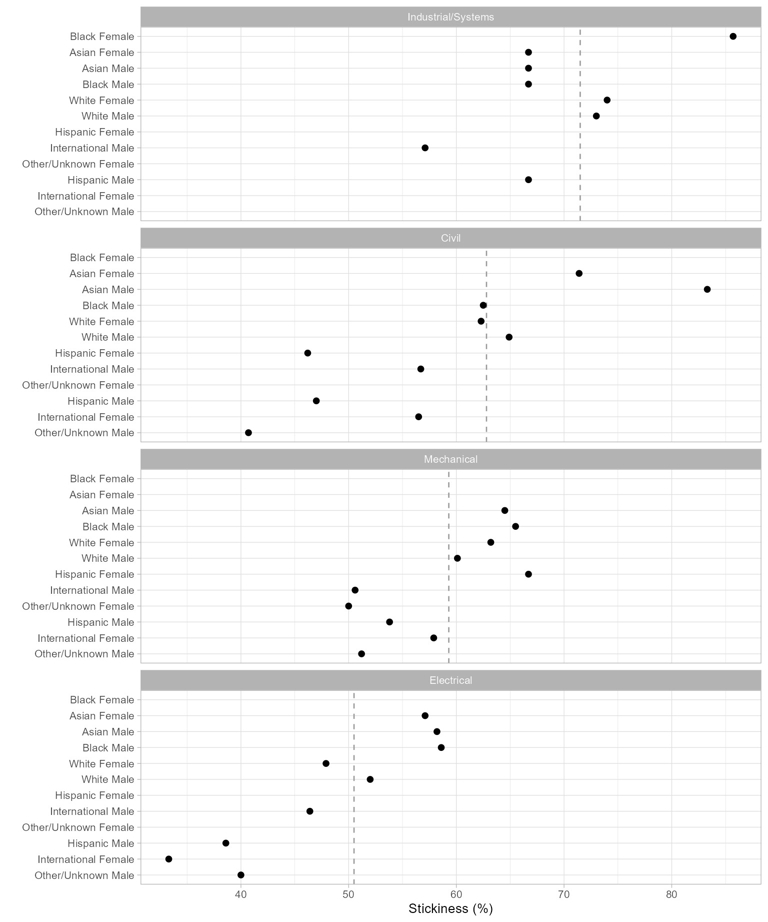

Figure 1: Program stickiness.

References

Cleveland, William S. 1993. Visualizing Data. Hobart Press.

Mount, John, and Nina Zumel. 2019. Coordinatized data: A fluid data specification. Win Vector LLC. http://winvector.github.io/FluidData/RowsAndColumns.html.

Ohland, Matthew, Marisa Orr, Richard Layton, Susan Lord, and Russell Long. 2012. “Introducing stickiness as a versatile metric of engineering persistence.” Proceedings of the Frontiers in Education Conference, 1–5.

Vignettes: data.table. 2026. Reference Semantics. https://r-datatable.com/articles/datatable-reference-semantics.html.