6 Graph basics

logo
Decline by Randall Munroe (xkcd.com) is licensed under CC BY-NC 2.5

6.1 Introduction

This tutorial is an introduction to ggplot2 adapted from Chapter 3 from [1]. If you already have R experience, you might still want to browse this section in case you find something new.

Prerequisites should be completed before proceeding. After that, the tutorial should take about an hour.

As you work through the tutorial, type a line or chunk of code then File > Save and run the script.
Confirm that your result matches the tutorial result.
The exercises give you chance to practice your new skills to learn by doing (but you knew that already)!

6.1.1 Download prepared data

Data sets used in the exercises have been prepared and saved in a .zip file in the workshop repository. The data are in .rds format, a native R format for single files that preserves variable types, including the order (if any) of factors.

Download the prepared_data.zip file from the workshop website with the following code.

You can copy and paste the code to the Console; you only have to run this once.
The destination file assumes you have a data directory in your project.

    zip_url <- paste0("https://github.com/MIDFIELDR/2021-asee-workshop/",
                      "raw/main/data/prepared_data.zip")
    download.file(zip_url, destfile = "data/prepared_data.zip")

If the download is unsuccessful

Navigate to the prepared_data.zip repository.
Click Download

Once the download is successful

Extract the compressed files from the downloaded .zip file.
Manually move the files into the top level of the workshop data folder. Your workshop data directory should now contain:

    data\
        hours_per_term.rds
        sat.rds
        stickiness.rds
        student_demogr.rds

6.1.2 Start a new script

Create a new script for this tutorial.

See Create a script if you need a refresher on creating, saving, and running an R script.
At the top of the script add a minimal header and install and load the packages indicated.

# Graph basics 
# Name 
# Date 

# Packages used in this tutorial
library("midfieldr")
library("midfielddata")
library("data.table")
library("ggplot2")
library("gapminder")

# Optional code to control data.table printing
options(
  datatable.print.nrows = 10,
  datatable.print.topn = 5,
  datatable.print.class = TRUE
)

# Load midfielddata data sets to use later
data(student)
data(term)

If you get an error like this one after running the script,

    Error in library("gapminder") : there is no package called 'gapminder'

then the package needs to be installed. If you need a refresher on installing packages, see Install CRAN packages. Once the missing package is installed, you can rerun the script.

6.2 Expected data structure

Data for analysis and graphing are often laid out in “block record” or “long” form with every key variable and response variable in their own columns [2]. Database designers call this a “denormalized” form; many R users would recognize it as the so-called “tidy” form [3].

We use this form regularly for preparing data for graphing using the ggplot2 package. The gapminder data we’re using in this tutorial is in block-record form. To view its help page, run

library("gapminder")
? gapminder

# Convert the data frame to a data.table structure 
gapminder <- data.table(gapminder)

And we can just type its name to see a few rows. Note at the top of each column under the column name, the class of the variable is shown: factor <fctr>, integer <int>, and double-precision <num>.

gapminder
#>           country continent  year lifeExp      pop gdpPercap
#>            <fctr>    <fctr> <int>   <num>    <int>     <num>
#>    1: Afghanistan      Asia  1952  28.801  8425333  779.4453
#>    2: Afghanistan      Asia  1957  30.332  9240934  820.8530
#>    3: Afghanistan      Asia  1962  31.997 10267083  853.1007
#>    4: Afghanistan      Asia  1967  34.020 11537966  836.1971
#>    5: Afghanistan      Asia  1972  36.088 13079460  739.9811
#>   ---                                                       
#> 1700:    Zimbabwe    Africa  1987  62.351  9216418  706.1573
#> 1701:    Zimbabwe    Africa  1992  60.377 10704340  693.4208
#> 1702:    Zimbabwe    Africa  1997  46.809 11404948  792.4500
#> 1703:    Zimbabwe    Africa  2002  39.989 11926563  672.0386
#> 1704:    Zimbabwe    Africa  2007  43.487 12311143  469.7093

x <- gapminder$continent
attributes(x)
#> $levels
#> [1] "Africa"   "Americas" "Asia"     "Europe"   "Oceania" 
#> 
#> $class
#> [1] "factor"

6.2.1 Exercise

Examine the student data from midfielddata. (Type its name in the console.)
How many variables? How many observations?
How many of the variables are numeric? How many are character type?
Is the data set in block-record form?
Check your work by comparing your result to the student help page (link below).

Help pages for more information:

6.3 Anatomy of a graph

ggplot() is a our basic plotting function. The data = ... argument assigns the data frame. The plot is empty because we haven’t mapped the data to coordinates yet.

ggplot(data = gapminder)

Next we use the mapping argument mapping = aes(...) to assign variables (column names) from the data frame to specific aesthetic properties of the graph such as the x-coordinate, the y-coordinate color, fill, etc.

Here we map continent (a categorical variable) to x and life expectancy (a quantitative variable) to y. To reduce the number of times we repeat lines of code, we can assign a name (life_exp) to the empty graph to which we can add layers later.

# Demonstrate aesthetic mapping
life_exp <- ggplot(data = gapminder, mapping = aes(x = continent, y = lifeExp))

To reduce typing, the first two arguments data and mapping are often used without naming them explicitly, e.g.,

# Demonstrate implicit data and mapping arguments
life_exp <- ggplot(gapminder, aes(x = continent, y = lifeExp))

If we print the graph by typing the name of the graph object (everything in R is an object), we get a graph with a range on each axis (from the mapping) but no data shown. We haven’t specified the type of visual encoding we want.

# Examine the result
life_exp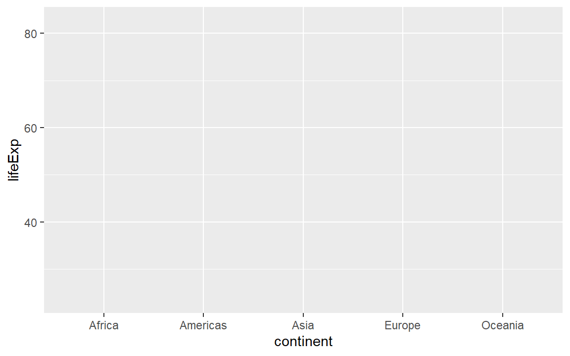

A box-and-whisker plot (or box plot) is designed for displaying the distribution of a single quantitative variable. The visual encoding is specified using the geom_boxplot() layer, where a “geom” is a geometric object. The geom_boxplot() function requires the quantitative variable assigned to y and the categorical variable (if any) to x.

# Demonstrate adding a geometric object 
life_exp <- life_exp + 
  geom_boxplot()

# Examine the result
life_exp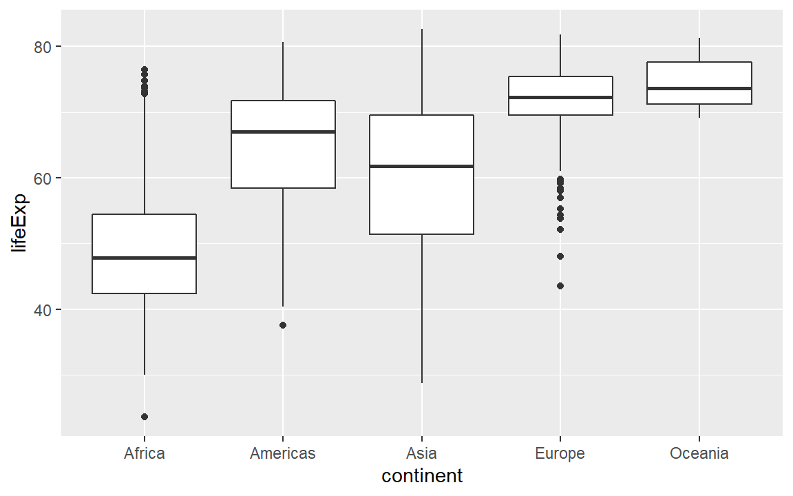

Notice that the default axis labels are the variables names from the data frame. We can edit those with another layer

# Demonstrate editing axis labels
life_exp <- life_exp + 
  labs(x = "Continent", y = "Life expectancy (years)")

# Examine the result
life_exp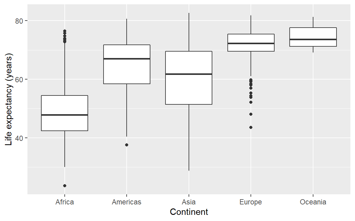

Next, we often want the categorical variable ordered by the quantitative variable instead of alphabetically. Because continent is a factor, we can use the reorder() function inside the aes() argument to order the boxplots by the median life expectancy per continent. For more information on ordering data, see Ordering factors.

# Demonstrate reordering a categorical variable 
life_exp + 
  aes(x = reorder(continent, lifeExp, median), y = lifeExp)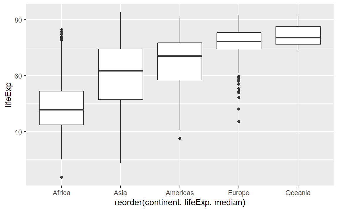

Summary. The basics steps for building up the layers of any graph:

assign the data frame
map variables (columns names) to aesthetic properties
choose geoms
adjust scales, labels, ordering, etc.

Lastly, while we separate the layers as we work to focus on that specific layer, the layers can always be written in a single code chunk, e.g,

ggplot(gapminder, aes(x = reorder(continent, lifeExp), y = lifeExp)) +
  geom_boxplot() +
  labs(x = "Continent", y = "Life expectancy (years)")

6.3.1 Exercise

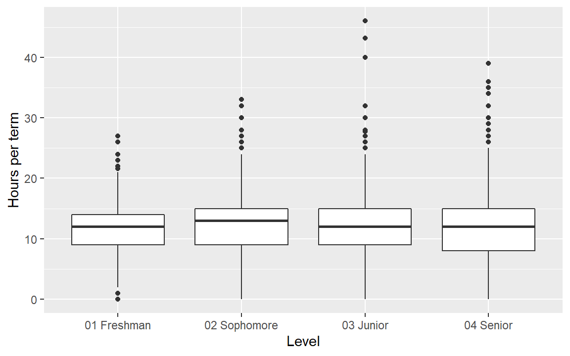
Examine the term data set from midfielddata.
Create a boxplot of the hours per term quantity conditioned by the student level.
What is the rational for leaving the categorical variable in its native order?
Check your work by comparing your result to the graph below.

Help pages for more information:

6.4 Layer: points

A two-dimensional scatterplot reveals the strength of the relationship between two quantitative variables. The ggplot geom for scatterplots is geom_point(). To illustrate a scatterplot, we graph life expectancy as a function of GDP.

life_gdp <- ggplot(gapminder, aes(x = gdpPercap, y = lifeExp)) +
  geom_point() +
  labs(x = "GDP per capita (USD)", y = "Life expectancy (years)")

life_gdp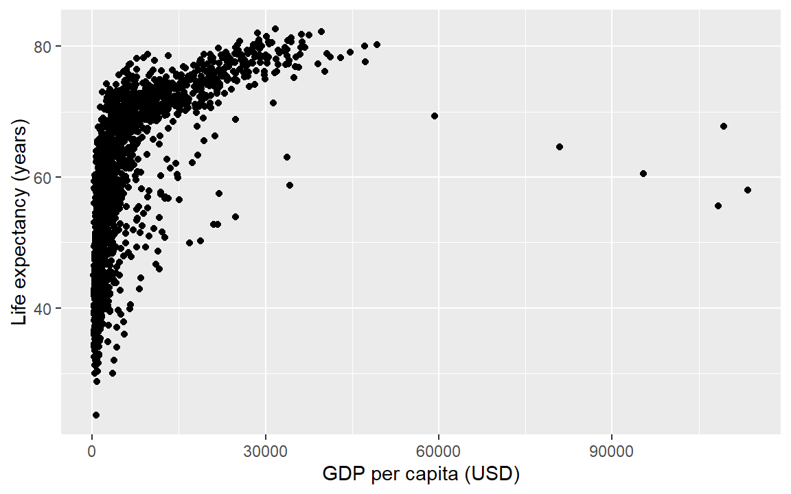

Help pages for more information:

geom_point()

6.5 Layer: smooth fit

Suppose you wanted a smooth fit curve, not necessarily linear. Add a geom_smooth() layer. The name loess (pronounced like the proper name Lois) is a nonparametric curve-fitting method based on local regression.

life_gdp + 
  geom_smooth(method = "loess", se = FALSE)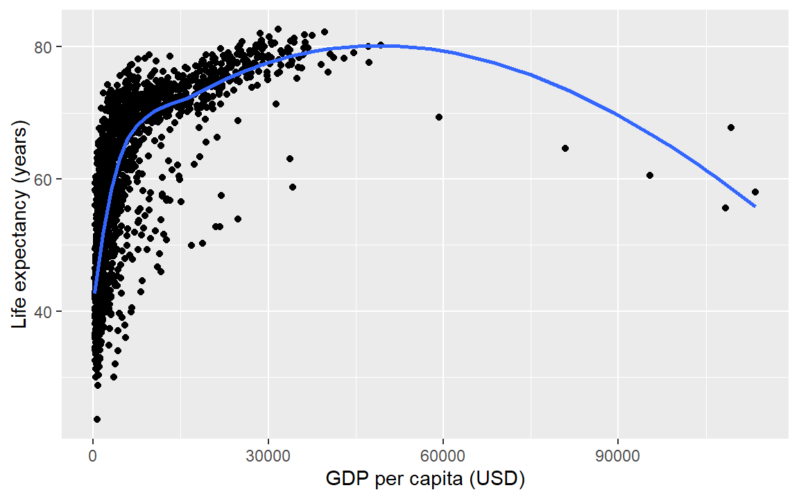

The se argument controls whether or not the confidence interval is displayed. Setting se = TRUE yields,

life_gdp + 
  geom_smooth(method = "loess", se = TRUE)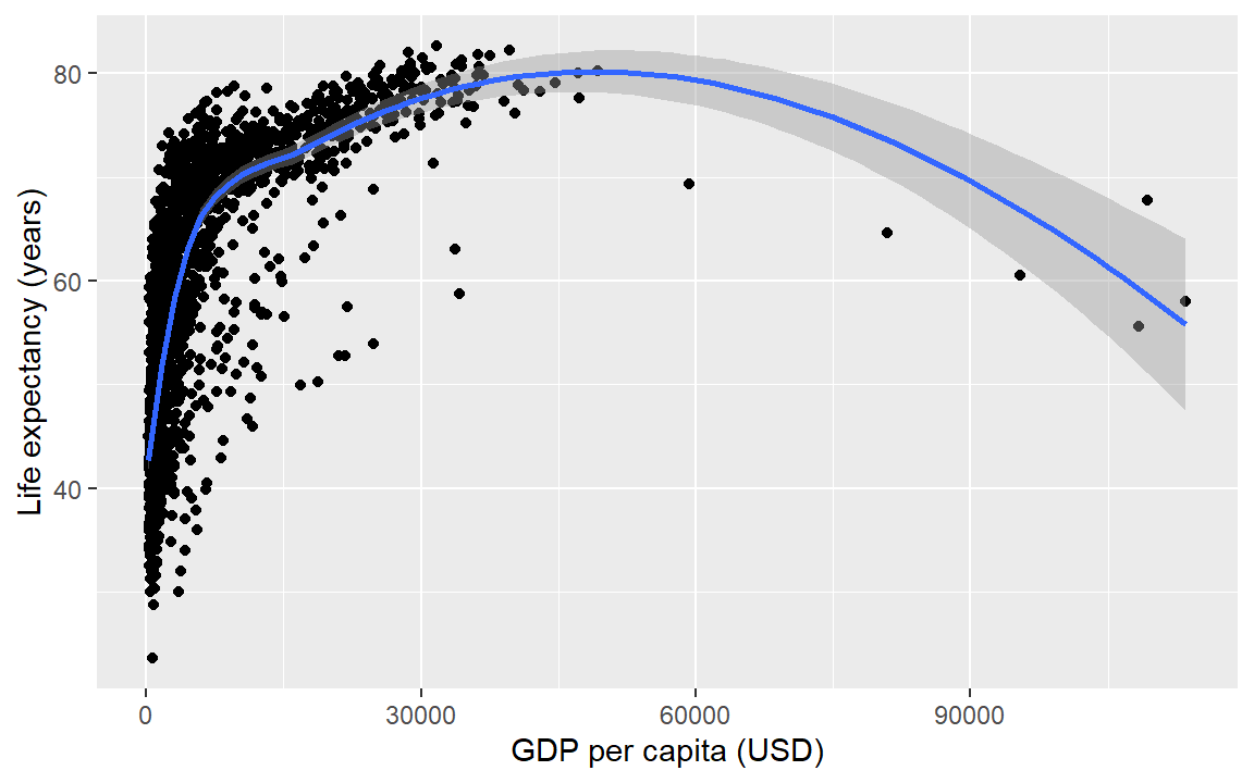

For a linear-fit layer, we change method to lm (short for linear model). The linear fit is not particularly good in this case, but now you know how to do one.

life_gdp + 
  geom_smooth(method = "lm", se = TRUE)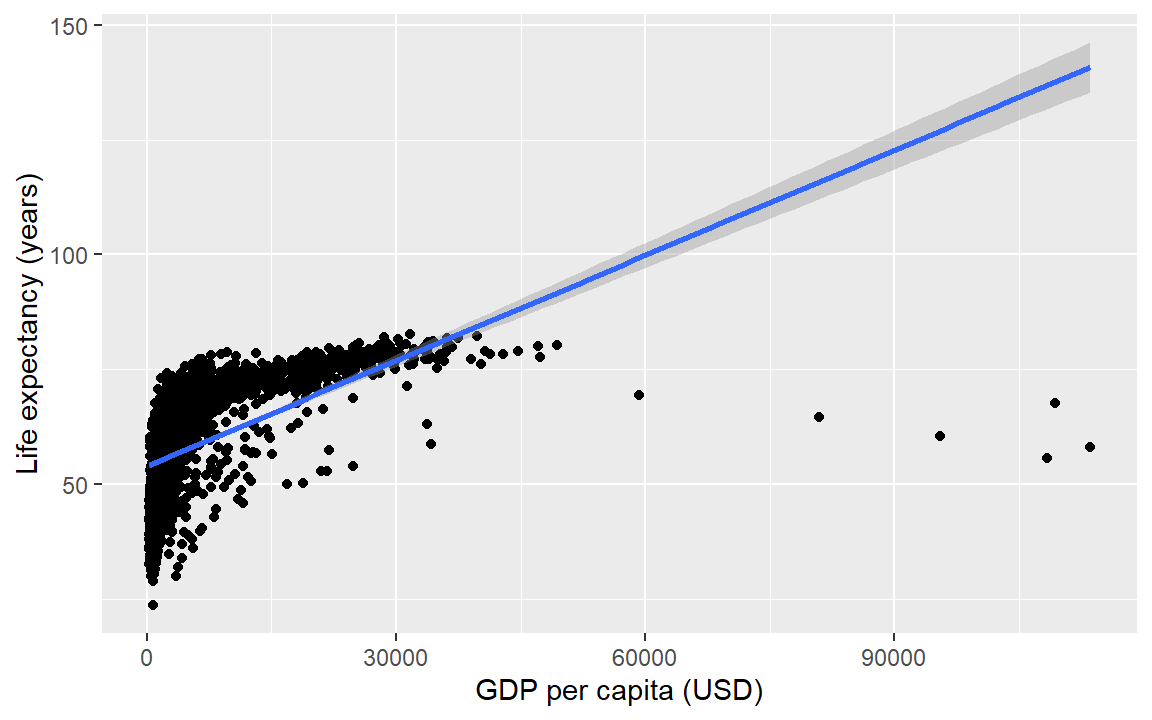

Help pages for more information:

geom_smooth()

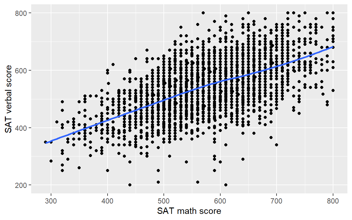
6.5.1 Exercise

A data set has been extracted from the midfieldr student table with a sample of 3000 student SAT scores. These data, sat.rds are part of the prepared data from the .zip files you downloaded earlier. Here we read the data in using readRDS().

# Prepared data from the downloaded zip file
sat <- readRDS("data/sat.rds")

Use the sat data and create a scatterplot of verbal scores sat_verbal as a function of math scores sat_math.
Add a loess fit.
Check your work by comparing your result to the graph below.

6.6 Layer: scale

We have orders of magnitude differences in the GDP per capita variable. To confirm, we can create a summary() of the gdpPercap variable. The output shows that the minimum is 241, the median 3532, and the maximum 113,523.

# statistical summary of one variable 
summary(gapminder[, gdpPercap])
#>     Min.  1st Qu.   Median     Mean  3rd Qu.     Max. 
#>    241.2   1202.1   3531.8   7215.3   9325.5 113523.1

In exploring a graph like this, it might be useful to add a layer that changes the horizontal scale to a log-base-10 scale.

life_gdp <- life_gdp +
  scale_x_continuous(trans = "log10")

Update the axis labels,

life_gdp <- life_gdp +
  labs(x = "GDP per capita, USD (log10 scale)", 
       y = "Life expectancy (years)")

life_gdp # display the graph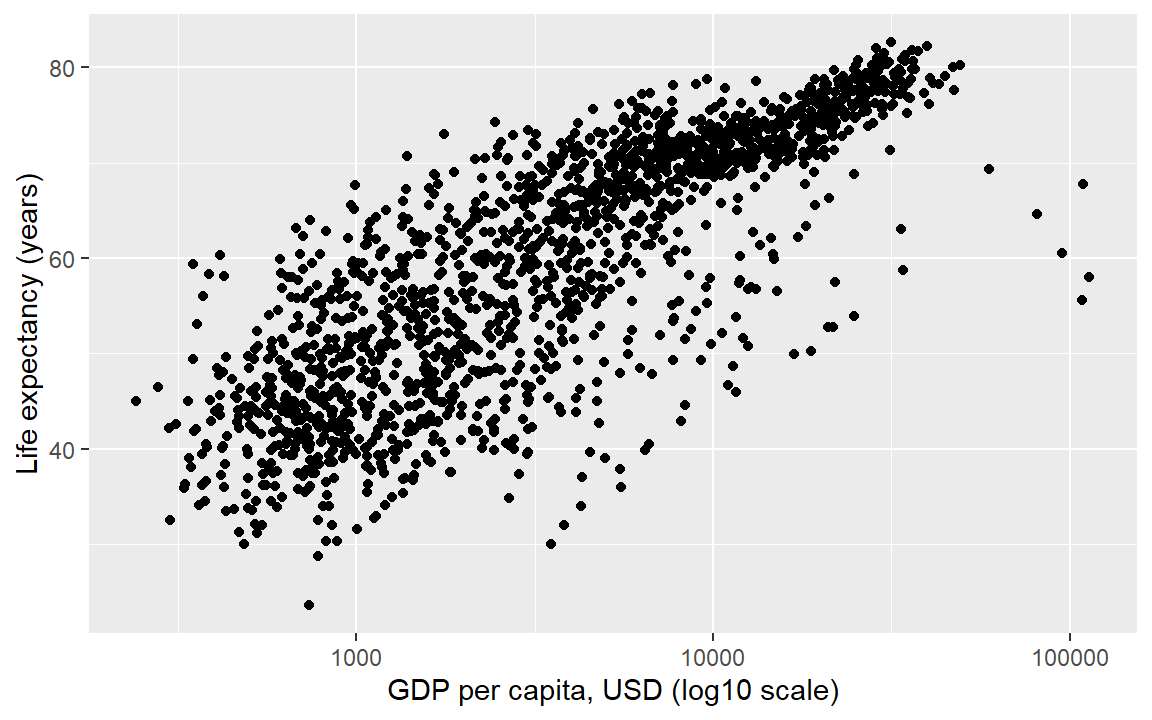

In summary, all the layers could have been be coded at once, for example,

ggplot(gapminder, aes(x = gdpPercap, y = lifeExp)) +
  geom_point() +
  scale_x_continuous(trans = "log10") +
  labs(x = "GDP per capita, USD (log10 scale)", 
       y = "Life expectancy (years)")

With all the layers in one place, we can see that we’ve coded all the basic steps, that is,

assign the data frame
map variables (columns names) to aesthetic properties
choose geoms
adjust scales, labels, ordering, etc.

6.6.1 Exercise

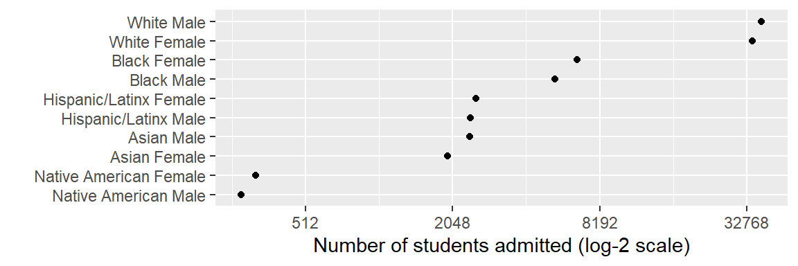
The prepared data you downloaded earlier includes the file student_demogr.rds. The data in this file is a summary of the midfieldr student table with the number of students by race/ethnicity and sex, omitting “International” and “Other/Unknown” race values. Again, we read the data in using readRDS().

# Prepared data from the downloaded zip file
student_demogr <- readRDS("data/student_demogr.rds")

Use the student_demogr data and reproduce the graph shown below.
Use a log-base-2 scale.
Omit the y-axis label by setting y = "" in the labs() argument.

Help pages for more information:

scale_x_continuous()

6.7 Mapping columns to aesthetics

Mappings in the aes() function of ggplot() can involve the names of variables (column s) only. So far, the only mappings we’ve used are from column names to an x or y aesthetic.

Another useful mapping is from a column name to the color argument, which then separates the data by the values of the categorical variable selected and automatically creates the appropriate legend.

Here we map the continent column to the color aesthetic, adding a third data variable to the display.

ggplot(gapminder, aes(x = gdpPercap, y = lifeExp, color = continent)) +
  geom_point() +
  scale_x_continuous(trans = "log10") +
  labs(x = "GDP per capita, USD (log10 scale)", 
       y = "Life expectancy (years)")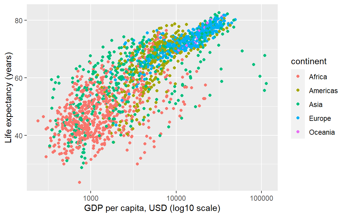

6.7.1 Exercise

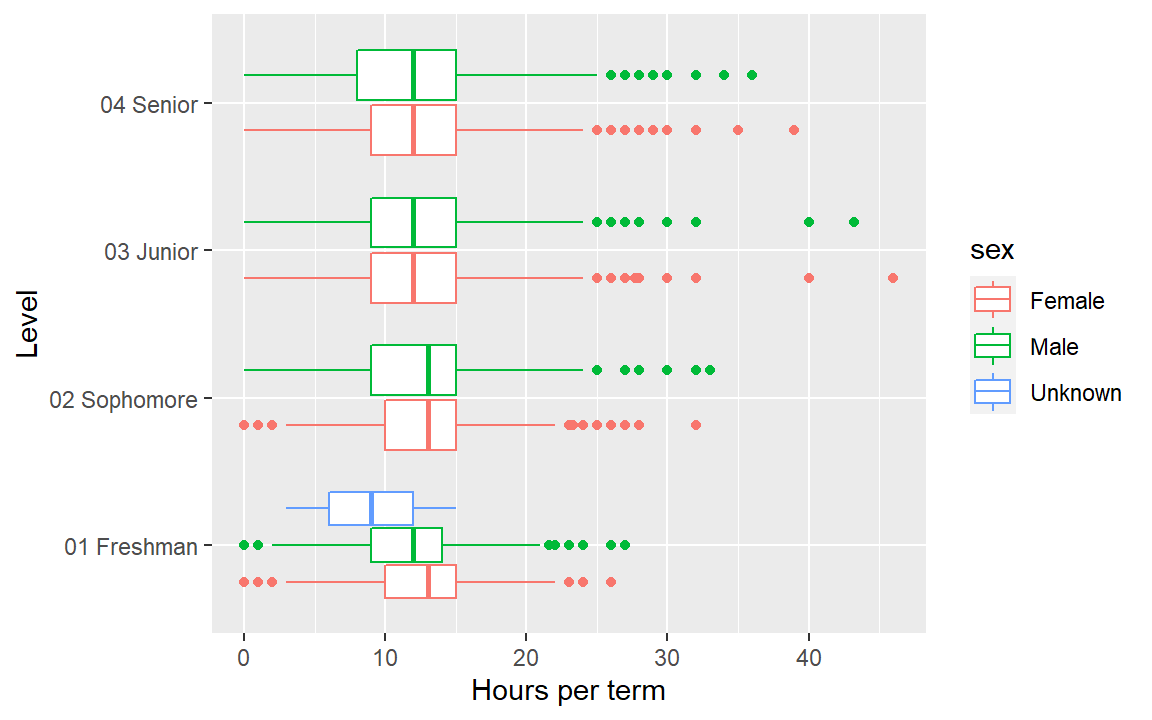
The prepared data you downloaded earlier includes the file hours_per_term.rds. Again, we read the data using readRDS().

hours_per_term <- readRDS("data/hours_per_term.rds")

Use hours_per_term data to create a boxplot of hours per term as a function of level.
Add a third column name to aes() to add sex by color to the graph.
Swap the x, y mapping to obtain a horizontal boxplot.
Check your work by comparing your result to the graph below.

Help pages for more information:

6.8 Layer: facets

In the earlier graph where we mapped continent to color, there was a lot of overprinting, making it difficult to compare the continents. Instead of using color to distinguish the continents, we can plot in different panels by continent.

The facet_wrap() layer separates the data into different panels (or facets). Like the aes() mapping, facet_wrap() is applied to a variable (column name) in the data frame.

life_gdp <- life_gdp + 
  facet_wrap(facets = vars(continent))

life_gdp # print the graph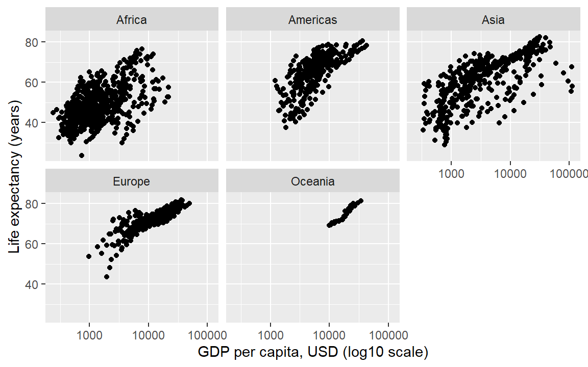

Comparisons are facilitated by having the facets appear in one column, by using the ncol argument of facet_wrap().

life_gdp <- life_gdp + facet_wrap(facets = vars(continent), ncol = 1)

life_gdp # print the graph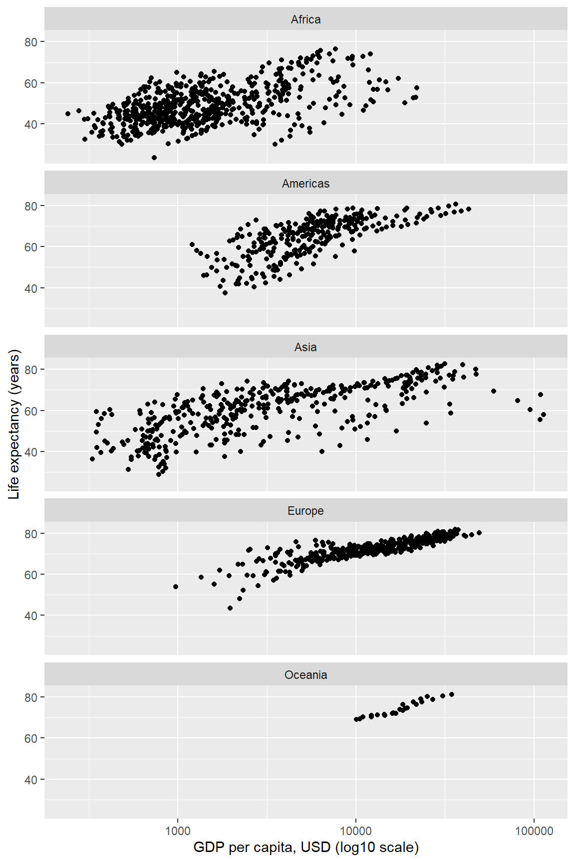

In a faceted display, all panels have identical scales (the default) to facilitate comparison. Again, all the layers could have been be coded at once, for example,

ggplot(gapminder, aes(x = gdpPercap, y = lifeExp)) +
  facet_wrap(facets = vars(continent), ncol = 1) +
  geom_point() +
  scale_x_continuous(trans = "log10") +
  labs(x = "GDP per capita, USD (log10 scale)", 
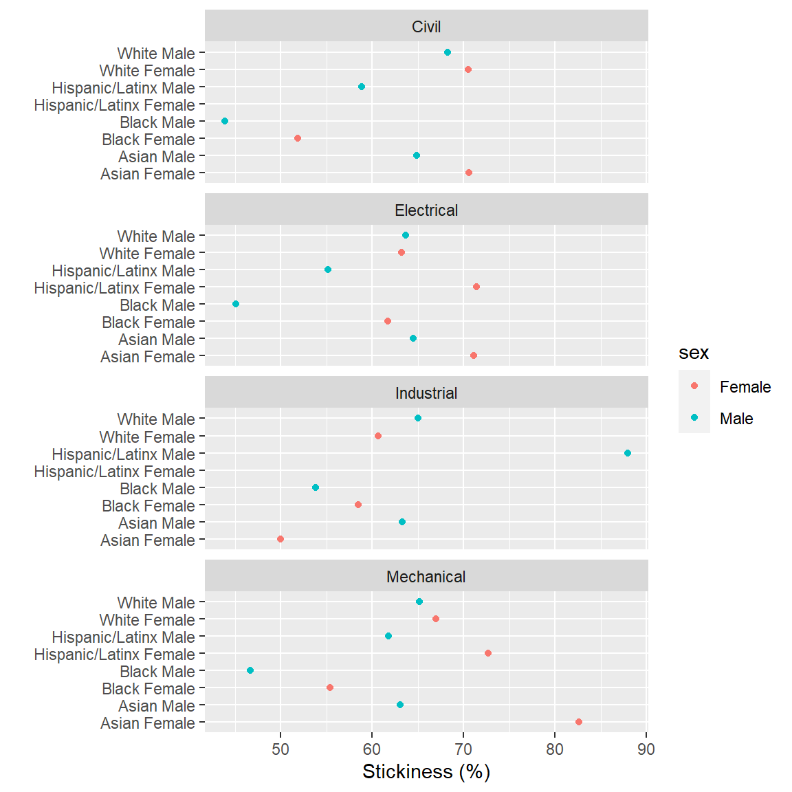
       y = "Life expectancy (years)")

6.8.1 Exercise

The prepared data you downloaded earlier includes the file stickiness.rds. Again, we read the data using readRDS().

stickiness <- readRDS("data/stickiness.rds")

Use the stickiness data frame and plot stickiness (x-axis) as a function of race/ethnicity/sex (y-axis) and faceted by program.
When that graph seems OK, add a third column name to aes() to add sex by color to the graph.
Check your work by comparing your result to the graph below.

Help pages for more information:

facet_wrap()

6.9 Ordering factors

Earlier, we used reorder() to order life expectancy boxplots by the increasing median life expectancy per continent. In general, we use reorder() to order every categorical variable we intend to display graphically.

A factor is special data structure in R for categorical variables. In a factor, the levels of the category—typically character strings—are known and fixed. However, factors are stored internally as integers—a critical design tool for meaningfully ordering the elements of a display involving categorical variables.

For example, reviewing again the gapminder data frame, we see that the first two columns are factors.

gapminder
#>           country continent  year lifeExp      pop gdpPercap
#>            <fctr>    <fctr> <int>   <num>    <int>     <num>
#>    1: Afghanistan      Asia  1952  28.801  8425333  779.4453
#>    2: Afghanistan      Asia  1957  30.332  9240934  820.8530
#>    3: Afghanistan      Asia  1962  31.997 10267083  853.1007
#>    4: Afghanistan      Asia  1967  34.020 11537966  836.1971
#>    5: Afghanistan      Asia  1972  36.088 13079460  739.9811
#>   ---                                                       
#> 1700:    Zimbabwe    Africa  1987  62.351  9216418  706.1573
#> 1701:    Zimbabwe    Africa  1992  60.377 10704340  693.4208
#> 1702:    Zimbabwe    Africa  1997  46.809 11404948  792.4500
#> 1703:    Zimbabwe    Africa  2002  39.989 11926563  672.0386
#> 1704:    Zimbabwe    Africa  2007  43.487 12311143  469.7093

A factor has at least two attributes, its class (all R objects have class) and its levels.

# Examine a factor variable 
x <- gapminder$continent

class(x)
#> [1] "factor"

levels(x)
#> [1] "Africa"   "Americas" "Asia"     "Europe"   "Oceania"

The levels are the character strings we see as data values in the data frame column. However, factors are stored in memory as type integer, as shown by the typeof() function.

# Factors are stored internally as integers
typeof(x)
#> [1] "integer"

If we unclass() the variable, we remove the class and reveal the hidden integers. For example, let’s first print out 64 values of continent,

# Data values are character strings
x[1:64]
#>  [1] Asia     Asia     Asia     Asia     Asia     Asia     Asia     Asia    
#>  [9] Asia     Asia     Asia     Asia     Europe   Europe   Europe   Europe  
#> [17] Europe   Europe   Europe   Europe   Europe   Europe   Europe   Europe  
#> [25] Africa   Africa   Africa   Africa   Africa   Africa   Africa   Africa  
#> [33] Africa   Africa   Africa   Africa   Africa   Africa   Africa   Africa  
#> [41] Africa   Africa   Africa   Africa   Africa   Africa   Africa   Africa  
#> [49] Americas Americas Americas Americas Americas Americas Americas Americas
#> [57] Americas Americas Americas Americas Oceania  Oceania  Oceania  Oceania 
#> Levels: Africa Americas Asia Europe Oceania

Then remove the class to reveal the hidden integers.

# But the levels are stored as integers
unclass(x[1:64])
#>  [1] 3 3 3 3 3 3 3 3 3 3 3 3 4 4 4 4 4 4 4 4 4 4 4 4 1 1 1 1 1 1 1 1 1 1 1 1 1 1
#> [39] 1 1 1 1 1 1 1 1 1 1 2 2 2 2 2 2 2 2 2 2 2 2 5 5 5 5
#> attr(,"levels")
#> [1] "Africa"   "Americas" "Asia"     "Europe"   "Oceania"

When factors are graphed, the integers determine the increasing order in which the levels are plotted. When we use reorder(), we are shuffling the mapping of integers to levels.

We can order the levels of continent by the median life expectancy per continent using,

x <- gapminder$continent
y <- gapminder$lifeExp
z <- reorder(x, y, median)

Examining the reordered factor z, notice the change in order of the levels in the printout. The levels are no longer in alphabetical order: the Americas and Asia have swapped positions. Asia is now mapped to the integer 2 where before it was mapped to 3.

levels(z)
#> [1] "Africa"   "Asia"     "Americas" "Europe"   "Oceania"

z[1:64]
#>  [1] Asia     Asia     Asia     Asia     Asia     Asia     Asia     Asia    
#>  [9] Asia     Asia     Asia     Asia     Europe   Europe   Europe   Europe  
#> [17] Europe   Europe   Europe   Europe   Europe   Europe   Europe   Europe  
#> [25] Africa   Africa   Africa   Africa   Africa   Africa   Africa   Africa  
#> [33] Africa   Africa   Africa   Africa   Africa   Africa   Africa   Africa  
#> [41] Africa   Africa   Africa   Africa   Africa   Africa   Africa   Africa  
#> [49] Americas Americas Americas Americas Americas Americas Americas Americas
#> [57] Americas Americas Americas Americas Oceania  Oceania  Oceania  Oceania 
#> Levels: Africa Asia Americas Europe Oceania

unclass(z[1:64])
#>  [1] 2 2 2 2 2 2 2 2 2 2 2 2 4 4 4 4 4 4 4 4 4 4 4 4 1 1 1 1 1 1 1 1 1 1 1 1 1 1
#> [39] 1 1 1 1 1 1 1 1 1 1 3 3 3 3 3 3 3 3 3 3 3 3 5 5 5 5
#> attr(,"levels")
#> [1] "Africa"   "Asia"     "Americas" "Europe"   "Oceania"

The purpose of this detailed examination is to lay the foundation for using reorder() to condition categorical variables for graphing. One of the most common applications is to order the panels and rows of a multi-facet graph. Panels (facets) by default are nearly always ordered alphabetically. In most cases, ordering the panels by the data improves the display.

In the next example, we again order the continents by the median life expectancy per continent, but here the ordering affects the order of the panels.

# Create a new memory location
dframe <- copy(gapminder)

# Order the levels of the factor 
dframe[, continent := reorder(continent, lifeExp, median)]

We graph using much the same code chunk as before with one addition. We add the as.table = FALSE argument to the facet_wrap() function. “Table-order” of panels is increasing from top to bottom; what we want is “graph-order,” increases (like a graph scale) from bottom to top.

ggplot(dframe, aes(x = gdpPercap, y = lifeExp)) +
  facet_wrap(facets = vars(continent), ncol = 1, as.table = FALSE) +
  geom_point() +
  scale_x_continuous(trans = "log10") +
  labs(x = "GDP per capita, USD (log10 scale)", 
       y = "Life expectancy (years)")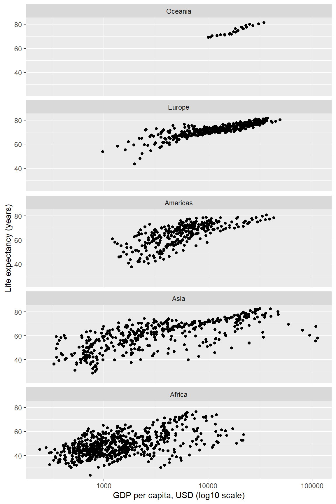

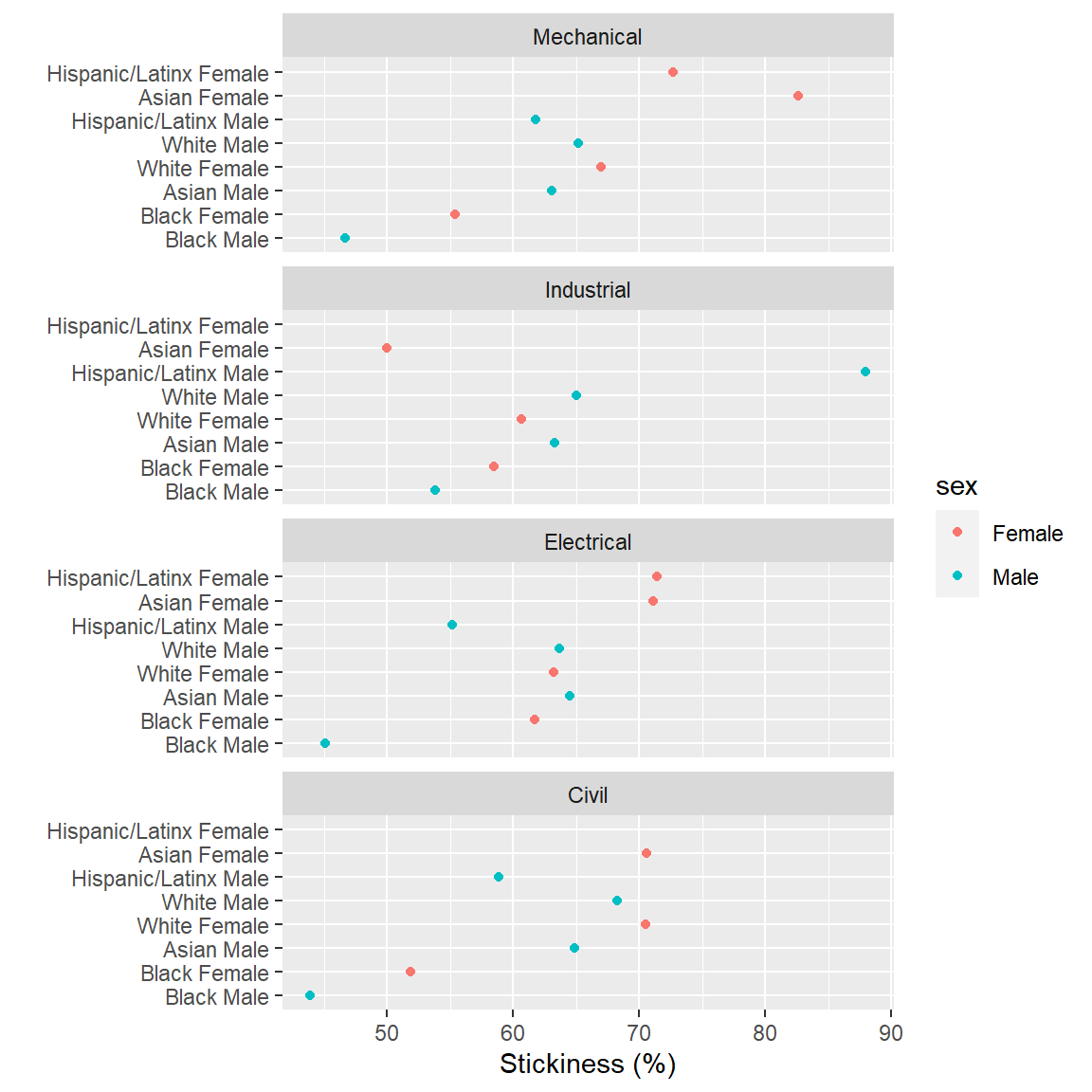
6.9.1 Exercise

Continue using the stickiness data frame from the previous section.

The race_sex and program columns are factors. Order both factors by the stickiness variable.
Use as.table to impose “graph-order” on the panels.
Check your work by comparing your result to the graph below.

Help pages for more information:

reorder()

6.10 Next steps

That concludes our brief introduction to graph basics using ggplot2. To continue, select your preferred next step in your progression.

▲ top of page