R basics

An introduction to key concepts in R.

License. This material is adapted from Getting started in R: Tinyverse edition by Bashir and Eddelbuettel (2018) which was licensed under CC BY-SA by ilustat. This adaptation and extension, R basics by Richard Layton, is licensed under CC BY-SA 2.0.

Preface

This guide gives you a flavor of what R can do for you. To get the most out of this guide, do the examples and exercises as you read along.

Experiment safely. Be brave and experiment with commands and options as it is an essential part of the learning process. Things can and will go “wrong”, like getting error messages or deleting things that you create. You can recover from most situations using “undo” ctrl Z (MacOS cmd Z) or restarting R with the RStudio menu Session > Restart R.

Before starting. Our tutorials assume that you

Have completed the Before you arrive instructions
Start your R session by launching the RStudio project you created, e.g., midfield-institute-2022.Rproj

If you are in an RStudio project, the project name appears in the upper left corner of the RStudio window. Your project directory (folder) should look something like this:

midfield-institute-2022\
    data\
    results\
    scripts\
    midfield-institute-2022.Rproj

Getting started

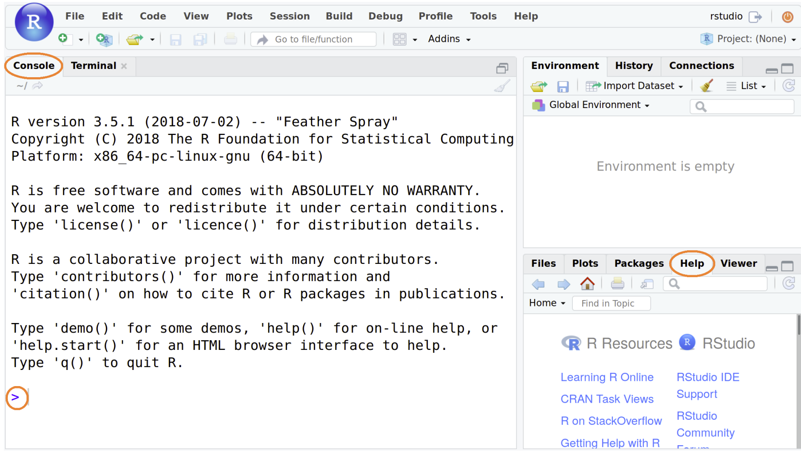
Starting R & RStudio. R starts automatically when you open RStudio with a screen similar to Figure 1. The console starts with information about the version number, license and contributors. The last line is a prompt (>) that indicates R is ready to do something.

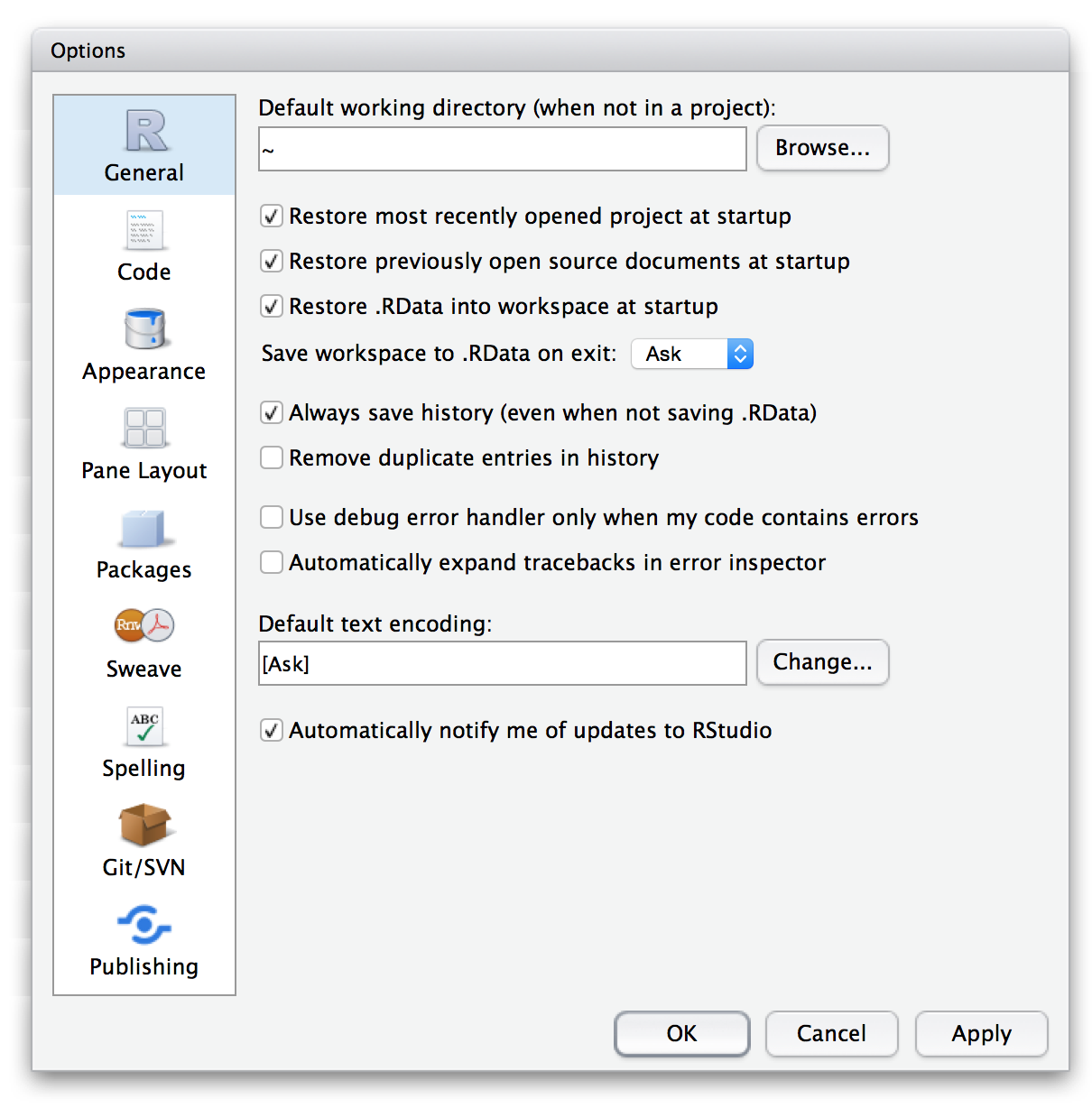
Figure 1: RStudio screenshot with Console on the left and Help tab in the bottom right

Quitting R & RStudio. When you quit RStudio you will be asked whether to Save workspace? with a yes or no option. If you choose Yes, your current workspace is restored the next time you open RStudio. But as long as you save your script, saving the workspace is unnecessary. I recommend you choose No.

To set No as the default option, from the RStudio menu select Tools > Global Options.

Un-check the box Restore .RData into workspace at startup
Set Save workspace to .RData on exit: to “Never”

Figure 2: RStudio global options default settings.

R help

R’s built-in help system is an essential part of finding solutions to your R programming problems.

help() function. From the R Console you can use the help() function or ?. For example, try the following two commands (which give the same result):

# view the function help page
help(mean)
? mean

Keyword search. To do a keyword search use the function apropos() with the keyword in double quotes (“keyword”) or single quote (‘keyword’). For example:

# keyword search 
apropos("mean")
#>  [1] ".colMeans"     ".rowMeans"     "colMeans"      "kmeans"       
#>  [5] "mean"          "mean.Date"     "mean.default"  "mean.difftime"
#>  [9] "mean.POSIXct"  "mean.POSIXlt"  "rowMeans"      "weighted.mean"

The lines of R output are labeled—here with [1], [5] , and [9]. These labels indicate the index or position of the first element in that line within the overall output (here, of length 12). Thus in this output vector, ".colMeans" has index 1, "mean" has index 5, and "mean.POSIXct" has index 9.

Help examples. Use the example() function to run the examples at the end of the help for a function:

# run the examples at the end of the help page
example(mean)
#> 
#> mean> x <- c(0:10, 50)
#> 
#> mean> xm <- mean(x)
#> 
#> mean> c(xm, mean(x, trim = 0.10))
#> [1] 8.75 5.50

Here, the output of the mean() example has length 2 (8.75 5.50). The label [1] indicates that the number 8.75 has index 1.

RStudio help. Rstudio provides search box in the Help tab to make your life easier (see Figure 1).

Online help. When you search online use [r] in your search terms, for example, “[r] linear regression”. Because we use data.table for data manipulation, I further recommend that you include data.table as a keyword, e.g., “[r][data.table] group and summarize”.

There is nearly always more than one solution to your problem—investigate the different options and try to use one whose arguments and logic you can follow. Limiting your browser’s search to the past year can sometimes eliminate out-of-date solutions.

Your turn
Answer

Try the following.

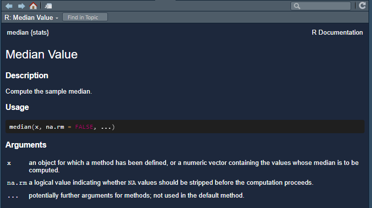
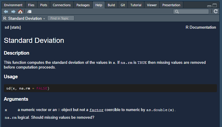
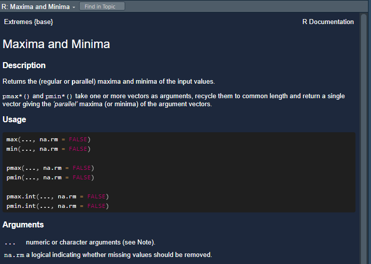
help(median)
? sd
? max

The following help pages should appear in the RStudio Help pane.

Warning. If an R command is not complete then R will show a plus sign (+) prompt on second and subsequent lines until the command syntax is correct.

Press the escape key (ESC) to break out.

Hint. To recall a previous command, put your cursor in the Console and use the up arrow key (↑). To go between previously typed commands use the up and down arrow (↓) keys. To modify or correct a command use the left (←) and right arrow (→) keys.

R scripts

I recommend that you write your lines of code in a script. Scripts can saved, edited, and run again and again.

Use File > New File > R Script to create a new R script
File > Save As… to name the file (I suggest 01-r-basics.R), then save it to the scripts directory
At the top of the script, add a minimal header, something like:

# R basics 
# your name 
# date

The hash symbol # denotes a comment in R, that is, a line that isn’t run. Comments are annotations to make the source code easier for humans to understand but are ignored by R.

Next,

Use library() to load packages used in the script.

# packages
library("midfieldr")

Note: In a code chunk like the one above, you can click on the “Copy to clipboard” icon in the upper right corner to enable quick copy and paste from this document to your script.

Run the script by clicking the Source button. Alternatively, you can use the keyboard shortcuts ctrl A (MacOS cmd A) to select all lines then ctrl Enter (MacOS cmd Return) to run all lines. (See the appendices for a table of useful keyboard shortcuts.)

If you see an error like this one,

    Error in library("midfieldr"): there is no package called 'midfieldr'

then you should install the missing package(s) and run the script again. You can review how to install a package here.

Use your script throughout the tutorial. When a new chunk of code is given,

Copy the line(s) of code into your script, save, and run.
Check your result by comparing it to the result in the tutorial.
Check what you’ve learned using the Your turn exercises.

R concepts

In R speak, scalars, vectors, variables and datasets are called objects. To create objects (things) we use the assignment operator (<-).

For example, the object height is assigned a value of 173 as follows,

# assign a value to a named object 
height <- 173

Typing the name alone prints out its value,

# view
height
#> [1] 173

In these notes, everything that comes back to us in the Console as the result of running a script is shown prefaced by #>.

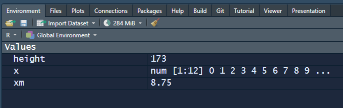
Objects in your R project workspace are listed in the RStudio Environment pane. At this point, we have three objects in the environment.

Warning: R is case sensitive. age and AgE are different:

# illustrating case-sensitivity 
age <- 10
AgE <- 50

# display result
age
#> [1] 10
AgE
#> [1] 50

New lines. R commands are usually separated by a new line but they can also be separated by a semicolon (not recommended).

# recommended style
name <- "Leo"
age  <- 25
city <- "Lisbon"

# views
name
#> [1] "Leo"
age
#> [1] 25
city
#> [1] "Lisbon"

# style not recommended 
name <- "Leo"; age <- 25; city <- "Lisbon"

# view
name; age; city
#> [1] "Leo"
#> [1] 25
#> [1] "Lisbon"

Comments. It is useful to put comments in your script—especially useful to the future you looking back at your script after several months.

R comments start with a hash sign (#). Everything after the hash to the end of the line is ignored by R.

# This comment line is ignored when run.

city # text after "#" is ignored.
#> [1] "Lisbon"

R as a calculator

You can use R as a calculator by typing in the Console. Try the following:

# type in the console
2 + 3
#> [1] 5

(5 * 11) / 4 - 7
#> [1] 6.75

7^3 # exponent
#> [1] 343

Other math functions. You can also use standard mathematical functions that are typically found on a scientific calculator.

trigonometric: sin(), cos(), tan(), etc.
rounding: abs(), ceiling(), floor(), round(), sign(), signif(), trunc()
logarithms and exponentials: log(), log10(), log2(), exp()

# type in the console

# square root
sqrt(2)
#> [1] 1.414214

# round down to nearest integer
floor(8.6178)
#> [1] 8

# round to 2 decimal places
round(8.6178, 2)
#> [1] 8.62

Your turn
Answer

What do the following pairs of examples do?

ceiling(18.33) and signif(9488, 2)
exp(1) and log10(1000)
sign(-2.9) and sign(32)
abs(-27.9) andabs(11.9)`

19 and 9500
2.718282 and 3
-1 and +1
27.9 and 11.9

More R concepts

From this point, please type the R code chunks in your script, save and run, and compare your results to those shown.

You can do some useful things using the assignment operator (<-), for example,

# assign dimensions
room_length <- 7.8
room_width  <- 6.4

# compute area
room_area <- room_length * room_width

# view
room_area
#> [1] 49.92

On coding style. We name R objects using so-called “snake-case”, that is, lowercase letters and numbers with underscores. You may of course use any style you are comfortable with.

Text objects. You can assign text to an object.

# assign text to an object
greeting <- "Hello world!"

# view
greeting
#> [1] "Hello world!"

Vectors. The objects presented so far have been scalars (single values). Working with vectors is where R shines best as they are the basic building blocks of datasets.

We can create a vector using the c() (combine values into a vector) function.

# a numeric vector
x1 <- c(26, 10, 4, 7, 41, 19)

# view
x1
#> [1] 26 10  4  7 41 19

# a character vector
x2 <- c("Peru", "Italy", "Cuba", "Ghana")

# view
x2
#> [1] "Peru"  "Italy" "Cuba"  "Ghana"

There are many other ways to create vectors, for example, rep() (replicate elements) and seq() (create sequences):

# repeat vector (2, 6, 7, 4) three times
r1 <- rep(c(2, 6, 7, 4), times = 3)

# view
r1
#>  [1] 2 6 7 4 2 6 7 4 2 6 7 4


# vector from -2 to 3 incremented by 0.5
s1 <- seq(from = -2, to = 3, by = 0.5)

# view
s1
#>  [1] -2.0 -1.5 -1.0 -0.5  0.0  0.5  1.0  1.5  2.0  2.5  3.0

Vector operations. You can do calculations on vectors, for example using x1 from above:

# multiply every element by 2
x1 * 2
#> [1] 52 20  8 14 82 38

# operation order: product, root, then round
round(sqrt(x1 * 2.6), 2)
#> [1]  8.22  5.10  3.22  4.27 10.32  7.03

Missing values. Missing values are coded as NA in R. For example,

# numeric vector with a missing value
x2 <- c(3, -7, NA, 5, 1, 1)

# view
x2
#> [1]  3 -7 NA  5  1  1

# character vector with a missing value
x3 <- c("rat", NA, "mouse", "hamster")

# view
x3
#> [1] "rat"     NA        "mouse"   "hamster"

Managing objects. Use function ls() to list the objects in your workspace. The rm() function deletes them.

# view objects in workspace
ls()
#>  [1] "age"         "AgE"         "city"        "greeting"    "height"     
#>  [6] "name"        "r1"          "room_area"   "room_length" "room_width" 
#> [11] "s1"          "x"           "x1"          "x2"          "x3"         
#> [16] "xm"

# remove objects
rm(x1, x2, x3, r1, s1, AgE, age)

# view result
ls()
#> [1] "city"        "greeting"    "height"      "name"        "room_area"  
#> [6] "room_length" "room_width"  "x"           "xm"

Your turn
Answer

Calculate the gross by adding the tax to net amount and round to the nearest integer.

net <- c(108.99, 291.42, 16.28, 62.29, 31.77)
tax <- c(22.89, 17.49, 0.98, 13.08, 6.67)

#> [1] 132 309  17  75  38

R functions and packages

R functions. We have already used some R functions (e.g. c(), mean(), rep(), sqrt(), round()). Most computation in R involves functions.

A function essentially has a name and a list of arguments separated by commas. For example:

# closer look at function arguments
seq(from = 5, to = 8, by = 0.4)
#> [1] 5.0 5.4 5.8 6.2 6.6 7.0 7.4 7.8

the function name is seq
the function has three arguments from (the start value), to (the end value), and by (the increment between values)
arguments are assigned values (using =) within the parentheses and are separated by commas

The seq() function has other arguments, documented in the help page. For example, we could use the argument length.out (instead of by) to fix the length of the sequence as follows:

# replacing `by` with `length.out` 
seq(from = 5, to = 8, length.out = 16)
#>  [1] 5.0 5.2 5.4 5.6 5.8 6.0 6.2 6.4 6.6 6.8 7.0 7.2 7.4 7.6 7.8 8.0

Custom functions. As you gain familiarity with R, you may want to learn how to construct your own custom functions, but that’s not an objective of our “basics” tutorials.

R packages. The basic R installation comes with over 2000 functions, but R can be extended further using contributed packages. Packages are like “apps” for R, containing functions, data, and documentation.

To see a list of functions and data sets bundled in a package, use the ls() function, e,g,

ls("package:midfieldr")
#>  [1] "add_completion_status"     "add_data_sufficiency"     
#>  [3] "add_timely_term"           "cip"                      
#>  [5] "filter_search"             "fye_predicted_start"      
#>  [7] "order_multiway_categories" "preprocess_fye"           
#>  [9] "study_mcid"                "study_observations"       
#> [11] "study_program_labels"      "study_results"            
#> [13] "toy_course"                "toy_degree"               
#> [15] "toy_student"               "toy_term"

Alternatively, in RStudio select the Packages tab and in its menu bar type the package name in the search box. In the pane, click on the package name. A help page opens listing all the functions and names of data sets in the package, e.g.,

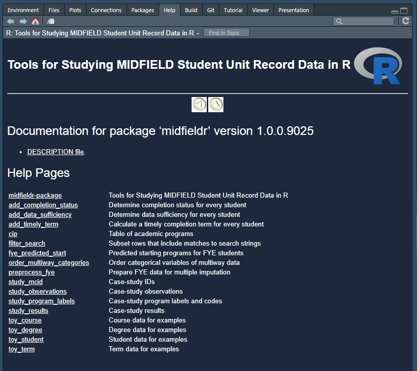
In MIDFIELD work, we use a small number of R packages:

midfieldr for tools to study student unit records
midfielddata for practice data
data.table for manipulating data
ggplot2 for charts

About R objects

Everything in R has class.

class(room_area)  # assigned earlier
#> [1] "numeric"

class(greeting)   # assigned earlier
#> [1] "character"

class(seq)        # R function 
#> [1] "function"

Certain actions will change the class of an object. Suppose we create a vector from the room_area and greeting objects.

x <- c(room_area, greeting)
x
#> [1] "49.92"        "Hello world!"

class(x)
#> [1] "character"

By concatenating a number and a character string, R changed the class of room area from “numeric” to “character” because all elements of a vector must have the same class.

Data frames. The most common class of data object we will use is the data frame: a two-dimensional array of rows and columns in R. All values in a column are of the same type (numerical, character, logical, etc.) but columns can be of different types.

For example, the data frame study_grad_rate that is bundled with midfieldr has two character columns and one numerical column.

# a data frame bundled with midfieldr
study_results
#>     program    sex            race ever grad stick
#>  1:      CE Female           Asian   16    9  56.2
#>  2:      CE Female           Black   49   15  30.6
#>  3:      CE Female Hispanic/Latinx   10    5  50.0
#>  4:      CE Female   International    1    0   0.0
#>  5:      CE Female   Other/Unknown    6    2  33.3
#>  6:      CE Female           White  304  156  51.3
#>  7:      CE   Male           Asian   34   17  50.0
#>  8:      CE   Male           Black   90   25  27.8
#>  9:      CE   Male Hispanic/Latinx   53   22  41.5
#> 10:      CE   Male   International   14    4  28.6
#> 11:      CE   Male Native American    7    1  14.3
#> 12:      CE   Male   Other/Unknown   13    4  30.8
#> 13:      CE   Male           White 1043  558  53.5
#> 14:      EE Female           Asian   36   14  38.9
#> 15:      EE Female           Black  145   58  40.0
#> 16:      EE Female Hispanic/Latinx   14    6  42.9
#> 17:      EE Female   International    8    3  37.5
#> 18:      EE Female Native American    3    0   0.0
#> 19:      EE Female   Other/Unknown    8    3  37.5
#> 20:      EE Female           White  173   55  31.8
#> 21:      EE   Male           Asian  189   86  45.5
#> 22:      EE   Male           Black  287   97  33.8
#> 23:      EE   Male Hispanic/Latinx   63   22  34.9
#> 24:      EE   Male   International   70   35  50.0
#> 25:      EE   Male Native American    8    1  12.5
#> 26:      EE   Male   Other/Unknown   27    9  33.3
#> 27:      EE   Male           White 1227  509  41.5
#> 28:     ISE Female           Asian   42   15  35.7
#> 29:     ISE Female           Black   93   43  46.2
#> 30:     ISE Female Hispanic/Latinx   13    8  61.5
#> 31:     ISE Female   International    6    3  50.0
#> 32:     ISE Female Native American    1    0   0.0
#> 33:     ISE Female   Other/Unknown    3    1  33.3
#> 34:     ISE Female           White  234  126  53.8
#> 35:     ISE   Male           Asian   65   34  52.3
#> 36:     ISE   Male           Black  103   46  44.7
#> 37:     ISE   Male Hispanic/Latinx   32   20  62.5
#> 38:     ISE   Male   International   24   12  50.0
#> 39:     ISE   Male Native American    1    0   0.0
#> 40:     ISE   Male   Other/Unknown    2    0   0.0
#> 41:     ISE   Male           White  494  263  53.2
#> 42:      ME Female           Asian   22   13  59.1
#> 43:      ME Female           Black   75   23  30.7
#> 44:      ME Female Hispanic/Latinx   10    4  40.0
#> 45:      ME Female   International    3    1  33.3
#> 46:      ME Female Native American    5    1  20.0
#> 47:      ME Female   Other/Unknown    8    4  50.0
#> 48:      ME Female           White  261  109  41.8
#> 49:      ME   Male           Asian  118   58  49.2
#> 50:      ME   Male           Black  202   65  32.2
#> 51:      ME   Male Hispanic/Latinx   76   29  38.2
#> 52:      ME   Male   International   36   16  44.4
#> 53:      ME   Male Native American   14    4  28.6
#> 54:      ME   Male   Other/Unknown   43   20  46.5
#> 55:      ME   Male           White 1776  918  51.7
#>     program    sex            race ever grad stick

class(study_results)
#> [1] "data.table" "data.frame"

The class() function reveals that this data.frame object is also a data.table object, which is an enhanced version of R’s standard data frame.

Your turn
Answer

For the following midfieldr objects, determine:

the class ofadd_timely_term
the class oftoy_student
the names of the variables in toy_term

# class of add_timely_term
#> [1] "function"

# class of toy_student
#> [1] "data.table" "data.frame"

# variables in toy_term
#> [1] "mcid" "institution" "term" "cip6" "level" "hours_term"

Everything in R has structure

str(room_area)  # assigned earlier
#>  num 49.9

str(greeting)         # assigned earlier
#>  chr "Hello world!"

str(seq)              # R function 
#> function (...)

str(study_results)
#> Classes 'data.table' and 'data.frame':   55 obs. of  6 variables:
#>  $ program: chr  "CE" "CE" "CE" "CE" ...
#>  $ sex    : chr  "Female" "Female" "Female" "Female" ...
#>  $ race   : chr  "Asian" "Black" "Hispanic/Latinx" "International" ...
#>  $ ever   : int  16 49 10 1 6 304 34 90 53 14 ...
#>  $ grad   : int  9 15 5 0 2 156 17 25 22 4 ...
#>  $ stick  : num  56.2 30.6 50 0 33.3 51.3 50 27.8 41.5 28.6 ...
#>  - attr(*, ".internal.selfref")=<externalptr>

Your turn
Answer

Use str() to determine

add_timely_term arguments
toy_student dimensions
toy_term numerical variables

dframe, midfield_term, span, sched_span
100 rows x 6 columns
hours_term

Keyboard shortcuts

If you are working in RStudio, you can see the menu of keyboard shortcuts using the menu Tools > Keyboard Shortcuts Help.

The shortcuts we use regularly include

Windows / Linux	Action	Mac OS
`ctrl shift K`	Compile R Markdown document	`cmd shift K`
`ctrl L`	Clear the RStudio Console	`ctrl L`
`ctrl shift C`	Comment/uncomment line(s)	`cmd shift C`
`ctrl X, C, V`	Cut, copy, paste	`cmd X, C, V`
`ctrl F`	Find in text	`cmd F`
`ctrl I`	Indent or re-indent lines od code	`cmd I`
`alt` –	Insert the assignment operator `<-`	`option` –
`ctrl alt B`	Run from begining to line	`cmd option B`
`ctrl alt E`	Run from line to end	`cmd option E`
`ctrl Enter`	Run selected line(s)	`cmd Return`
`ctrl S`	Save	`cmd S`
`ctrl A`	Select all text	`cmd A`
`ctrl Z`	Undo	`cmd Z`

References

Bashir, S., & Eddelbuettel, D. (2018). Getting started in R: Tinyverse edition. https://eddelbuettel.github.io/gsir-te/Getting-Started-in-R.pdf